作业要求:
电信公司希望针对客户的信息预测其流失可能性,数据存放在“telecom_churn.csv”中。
1、分析思路:
在对客户流失与否的影响因素进行模型研究之前,首先对各解释变量与被解释变量进行两变量独立性分析,
以初步判断影响流失的因素,进而建立客户流失预测模型
主要变量说明如下:
#subscriberID="个人客户的ID"
#churn="是否流失:1=流失";
#Age="年龄"
#incomeCode="用户居住区域平均收入的代码"
#duration="在网时长"
#peakMinAv="统计期间内最高单月通话时长"
#peakMinDiff="统计期间结束月份与开始月份相比通话时长增加数量"
#posTrend="该用户通话时长是否呈现出上升态势:是=1"
#negTrend="该用户通话时长是否呈现出下降态势:是=1"
#nrProm="电话公司营销的数量"
#prom="最近一个月是否被营销过:是=1"
#curPlan="统计时间开始时套餐类型:1=最高通过200分钟;2=300分钟;3=350分钟;4=500分钟"
#avPlan="统计期间内平均套餐类型"
#planChange="统计期间是否更换过套餐:1=是"
#posPlanChange="统计期间是否提高套餐:1=是"
#negPlanChange="统计期间是否降低套餐:1=是"
#call_10086="拨打10086的次数"
2、作业安排:
2.1 基础知识:
1)作了一次营销活动,营销了1000人 。事后统计结果,120人购买,其余人没有购买。请分别用矩估计法、极大似然估计法计算这个随机事件分布的参数(提示:该随机事件服从伯努利分布)
2)推导线性回归参数估计的最小二乘、矩估计、极大似然估计,推导逻辑回归的极大似然估计公式。线性回归和逻辑回归的极大似然法哪个可以得到
显性的公式解,哪个需要使用迭代法求解?解释极大似然法求解过程中用到的牛顿迭代法、随机梯度法的做法。
3)解释统计学习算法中超参的概念,请问目前统计方法中学习的线性回归、逻辑回归中涉及超参了吗?岭回归和Laso算法中的超参分别是什么?超参的作用是什么?统计学习算法中如何确定最优超参的取值?
4)比较统计分析法和统计学习(即机器学习)得到最优模型的思路。
5)二分类模型中(比如逻辑回归)的评估模型优劣的决策类和排序类评估指标分别包括哪些指标?
2.2 案例解答步骤如下:
1)两变量分析:检验该用户通话时长是否呈现出上升态势(posTrend)对流失(churn) 是否有预测价值
2)首先将原始数据拆分为训练和测试数据集,使用训练数据集建立在网时长对流失的逻辑回归,使用测试数据集制作混淆矩阵(阈值为0.5),提供准
确性、召回率指标,提供ROC曲线和AUC。
3)使用向前逐步法从其它备选变量中选择变量,构建基于AIC的最优模型,绘制ROC曲线,同时检验模型的膨胀系数。
4)使用岭回归和Laso算法重建第三步中的模型,使用交叉验证法确定惩罚参数(C值)。并比较步骤四中Laso算法得到的模型和第三步得到的模型的差异。
#%%

import pandas as pd

import seaborn as sns

import os

import numpy as np


os.chdir(r'D:\Learningfile\天善学院\280_Ben_八大直播八大案例配套课件\提交-第五讲:Logistic回归构建初始信用评级和分类模型检验\作业')

data=pd.read_csv('telecom_churn.csv')


data.head(5)


#%%

#1)两变量分析:检验该用户通话时长是否呈现出上升态势(posTrend)对流失(churn) 是否有预测价值

from scipy import stats

crosstable=pd.crosstab(data.posTrend,data.churn,margins=True)


def perCov(ser):

    return ser/ser[-1]


crosstable.apply(perCov,axis=1)


print('''chisq=%6.4f

      p-value=%6.4f

      dof=%i

      expected freq=%s'''% stats.chi2_contingency(crosstable.iloc[:2,:2]))
chisq=158.4433
p-value=0.0000
dof=1
expected freq=[[ 1013.24025411 805.75974589]
[ 915.75974589 728.24025411]]
#%%

#2)首先将原始数据拆分为训练和测试数据集,使用训练数据集建立在网时长对流失的逻辑回归,

#使用测试数据集制作混淆矩阵(阈值为0.5),提供准确性、召回率指标,提供ROC曲线和AUC。


train = data.sample(frac=0.7, random_state=0).copy()

test = data[~ data.index.isin(train.index)].copy()

print(' 训练集样本量: %i \n 测试集样本量: %i' %(len(train), len(test)))

#%%

#建模

import statsmodels.formula.api as smf

import statsmodels.api as sm


lg = smf.glm('churn ~ duration', data=train,

             family=sm.families.Binomial(sm.families.links.logit)).fit()

lg.summary()

#%%

train['proba'] = lg.predict(train)

test['proba'] = lg.predict(test)


test['proba'].head(10)

#%%

#设定阈值为0.5

test['prediction'] = (test['proba'] > 0.5).astype('int')

#混淆矩阵

crosstable2=pd.crosstab(test.churn, test.prediction, margins=True)

print(crosstable2)

#%%

#准确性

accuracy=(crosstable2.iloc[0,0]+crosstable2.iloc[1,1])/crosstable2.iloc[2,2]

print('准确性为:%s'% accuracy)

#召回率

recall=crosstable2.iloc[1,1]/crosstable2.iloc[2,1]

print('召回率为:%s' % recall)

'''

#acc

acc = sum(test['prediction'] == test['churn']) /np.float(len(test))

print('The accurancy is %.2f' %acc)

'''

#%%

#绘制ROC曲线

import sklearn.metrics as metrics

import matplotlib.pyplot as plt

fpr_test, tpr_test, th_test = metrics.roc_curve(test.churn, test.proba)

fpr_train, tpr_train, th_train = metrics.roc_curve(train.churn, train.proba)


plt.figure(figsize=[3, 3])

plt.plot(fpr_test, tpr_test, 'b--')

plt.plot(fpr_train, tpr_train, '')

plt.title('ROC curve')

plt.xlabel('fpr')

plt.ylabel('tpr')

plt.show()

#%%

#auc

print('AUC = %.4f' %metrics.auc(fpr_test, tpr_test))

#%%
准确性为:0.757459095284
召回率为:0.714555765595
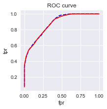
AUC = 0.8752
#3)使用向前逐步法从其它备选变量中选择变量,构建基于AIC的最优模型,绘制ROC曲线,同时检验模型的膨胀系数。

# 向前法

def forward_select(data, response):

    remaining = set(data.columns)

    remaining.remove(response)

    selected = []

    current_score, best_new_score = float('inf'), float('inf')

    while remaining:

        aic_with_candidates=[]

        for candidate in remaining:

            formula = "{} ~ {}".format(

                response,' + '.join(selected + [candidate]))

            aic = smf.glm(

                formula=formula, data=data,

                family=sm.families.Binomial(sm.families.links.logit)

            ).fit().aic

            aic_with_candidates.append((aic, candidate))

        aic_with_candidates.sort(reverse=True)

        best_new_score, best_candidate=aic_with_candidates.pop()

        if current_score > best_new_score:

            remaining.remove(best_candidate)

            selected.append(best_candidate)

            current_score = best_new_score

            print ('aic is {},continuing!'.format(current_score))

        else:

            print ('forward selection over!')

            break


    formula = "{} ~ {} ".format(response,' + '.join(selected))

    print('final formula is {}'.format(formula))

    model = smf.glm(

        formula=formula, data=data,

        family=sm.families.Binomial(sm.families.links.logit)

    ).fit()

    return(model)


#%%

#只选取连续变量进行建模,不要问为什么不用分类变量,WOE还不会

candidates = ['churn','AGE','incomeCode','duration','peakMinAv','peakMinDiff','nrProm','call_10086']

data_for_select = train[candidates]


lg_m1 = forward_select(data=data_for_select, response='churn')

lg_m1.summary()


#%%

#ROC曲线

train['proba'] = lg_m1.predict(train)

test['proba'] = lg_m1.predict(test)

import sklearn.metrics as metrics


fpr_test, tpr_test, th_test = metrics.roc_curve(test.churn, test.proba)

fpr_train, tpr_train, th_train = metrics.roc_curve(train.churn, train.proba)


plt.figure(figsize=[3, 3])

plt.plot(fpr_test, tpr_test, 'b--')

plt.plot(fpr_train, tpr_train, '')

plt.xlabel('fpr')

plt.ylabel('tpr')

plt.title('ROC curve')

plt.show()

#%%

print('AUC = %.4f' %metrics.auc(fpr_test, tpr_test))

#%%

def vif(df, col_i):

    from statsmodels.formula.api import ols


    cols = list(df.columns)

    cols.remove(col_i)

    cols_noti = cols

    formula = col_i + '~' + '+'.join(cols_noti)

    r2 = ols(formula, df).fit().rsquared

    return 1. / (1. - r2)

# In[18]:

candidates = ['churn','AGE','incomeCode','duration','peakMinAv','peakMinDiff','nrProm','call_10086']

exog = train[candidates].drop(['churn'], axis=1)


for i in exog.columns:

    print(i, '\t', vif(df=exog, col_i=i))
===============================================================================
coef std err z P>|z| [0.025 0.975]
-------------------------------------------------------------------------------
Intercept 3.1919 0.246 12.968 0.000 2.709 3.674
duration -0.2461 0.012 -20.694 0.000 -0.269 -0.223
peakMinDiff -0.0033 0.000 -8.946 0.000 -0.004 -0.003
call_10086 -0.7148 0.113 -6.299 0.000 -0.937 -0.492
AGE -0.0211 0.004 -5.073 0.000 -0.029 -0.013
incomeCode 0.0074 0.003 2.237 0.025 0.001 0.014
peakMinAv 0.0006 0.000 1.491 0.136 -0.000 0.001
===============================================================================
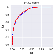
AUC = 0.8907
膨胀系数:
AGE 1.0557085932
incomeCode 1.0155921115
duration 1.04794631408
peakMinAv 1.04251995811
peakMinDiff 1.02771509732
nrProm 1.00189931029
call_10086 1.01726410895
#%%

#4)使用岭回归和Laso算法重建第三步中的模型,使用交叉验证法确定惩罚参数(C值)。

#并比较步骤四中Laso算法得到的模型和第三步得到的模型的差异。

#这里数据并未进行标准化

from sklearn.linear_model import Lasso

lasso=Lasso()

lasso.fit(exog,train['churn'])


#%%

import numpy as np

np.sum(lasso.coef_ !=0)

#%%

lasso_0 = Lasso(0)

lasso_0.fit(exog,train['churn'])

np.sum(lasso_0.coef_ != 0)

#%%

from sklearn.linear_model import LassoCV

lassocv=LassoCV()

lassocv.fit(exog,train['churn'])


print('alpha:',lassocv.alpha_)


print('变量权重:',lassocv.coef_)


#%%

from sklearn.linear_model import RidgeCV

rcv = RidgeCV(alphas=np.array([15.65,15.7, 15.75,15.8, 15.85]))

rcv.fit(exog,train['churn'])

rcv.alpha_

#%%

rcv.coef_
Lasso(alpha=1.0, copy_X=True, fit_intercept=True, max_iter=1000,
normalize=False, positive=False, precompute=False, random_state=None,
selection='cyclic', tol=0.0001, warm_start=False)
lassocv.alpha_: 0.023769813127661781
array([ -3.17191588e-03, 1.00149508e-03, -2.21743939e-02,
8.83592822e-05, -5.01785645e-04, 0.00000000e+00,
-1.33776368e-02])
======================================================
rcv.alpha_
Out[26]: 15.699999999999999
array([ -3.25960473e-03, 1.11183951e-03, -2.18431048e-02,
7.84930886e-05, -4.97128482e-04, 3.80187351e-03,
-1.08941057e-01])