
前言
在写代码前,先简单的过一下SVM的基本原理,如下:
SVM(support vector machine)简单的说是一个分类器,并且是二类分类器。
Vector:通俗说就是点,或是数据。
Machine:也就是classifier,也就是分类器。
SVM作为传统机器学习的一个非常重要的分类算法,它是一种通用的前馈网络类型,最早是由Vladimir N.Vapnik 和 Alexey Ya.Chervonenkis在1963年提出,目前的版本(soft margin)是Corinna Cortes 和 Vapnik在1993年提出,1995年发表。深度学习(2012)出现之前,SVM被认为是机器学习中近十几年最成功表现最好的算法。
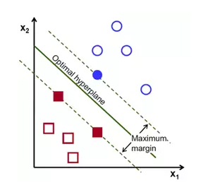
给定训练样本,支持向量机建立一个超平面作为决策曲面,使得正例和反例的隔离边界最大化。
决策曲面的初步理解可以参考如下过程,(来自:http://blog.csdn.net/jcjx0315/article/details/61929439)
1)如下图想象红色和蓝色的球为球台上的桌球,我们首先目的是找到一条曲线将蓝色和红色的球分开,于是我们得到一条黑色的曲线。

图一.
2) 为了使黑色的曲线离任意的蓝球和红球距离(也就是我们后面要提到的margin)最大化,我们需要找到一条最优的曲线。如下图,
图二.
3) 想象一下如果这些球不是在球桌上,而是被抛向了空中,我们仍然需要将红色球和蓝色球分开,这时就需要一个曲面,而且我们需要这个曲面仍然满足跟所有任意红球和蓝球的间距的最大化。需要找到的这个曲面,就是我们后面详细了解的最优超平面。


4) 离这个曲面最近的红色球和蓝色球就是Support Vector。
详细的原理请看之前的文章:
......
更多文章点击站内搜索链接:
python源码:
原文链接:https://www.cnblogs.com/buzhizhitong/p/6089070.html
# -*- coding: utf-8 -*-
"""
Created on Tue Nov 22 11:24:22 2016
@author: Administrator
"""
# Mathieu Blondel, September 2010
# License: BSD 3 clause
import numpy as np
from numpy import linalg
import cvxopt
import cvxopt.solvers
def linear_kernel(x1, x2):
return np.dot(x1, x2)
def polynomial_kernel(x, y, p=3):
return (1 + np.dot(x, y)) ** p
def gaussian_kernel(x, y, sigma=5.0):
return np.exp(-linalg.norm(x-y)**2 / (2 * (sigma ** 2)))
class SVM(object):
def __init__(self, kernel=linear_kernel, C=None):
self.kernel = kernel
self.C = C
if self.C is not None: self.C = float(self.C)
def fit(self, X, y):
n_samples, n_features = X.shape
# Gram matrix
K = np.zeros((n_samples, n_samples))
for i in range(n_samples):
for j in range(n_samples):
K[i,j] = self.kernel(X[i], X[j])
P = cvxopt.matrix(np.outer(y,y) * K)
q = cvxopt.matrix(np.ones(n_samples) * -1)
A = cvxopt.matrix(y, (1,n_samples))
b = cvxopt.matrix(0.0)
if self.C is None:
G = cvxopt.matrix(np.diag(np.ones(n_samples) * -1))
h = cvxopt.matrix(np.zeros(n_samples))
else:
tmp1 = np.diag(np.ones(n_samples) * -1)
tmp2 = np.identity(n_samples)
G = cvxopt.matrix(np.vstack((tmp1, tmp2)))
tmp1 = np.zeros(n_samples)
tmp2 = np.ones(n_samples) * self.C
h = cvxopt.matrix(np.hstack((tmp1, tmp2)))
# solve QP problem
solution = cvxopt.solvers.qp(P, q, G, h, A, b)
# Lagrange multipliers
'''
数组的flatten和ravel方法将数组变为一个一维向量(铺平数组)。
flatten方法总是返回一个拷贝后的副本,
而ravel方法只有当有必要时才返回一个拷贝后的副本(所以该方法要快得多,尤其是在大数组上进行操作时)
'''
a = np.ravel(solution['x'])
# Support vectors have non zero lagrange multipliers
'''
这里a>1e-5就将其视为非零
'''
sv = a > 1e-5 # return a list with bool values
ind = np.arange(len(a))[sv] # sv's index
self.a = a[sv]
self.sv = X[sv] # sv's data
self.sv_y = y[sv] # sv's labels
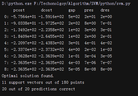
print("%d support vectors out of %d points" % (len(self.a), n_samples))
# Intercept
'''
这里相当于对所有的支持向量求得的b取平均值
'''
self.b = 0
for n in range(len(self.a)):
self.b += self.sv_y[n]
self.b -= np.sum(self.a * self.sv_y * K[ind[n],sv])
self.b /= len(self.a)
# Weight vector
if self.kernel == linear_kernel:
self.w = np.zeros(n_features)
for n in range(len(self.a)):
# linear_kernel相当于在原空间,故计算w不用映射到feature space
self.w += self.a[n] * self.sv_y[n] * self.sv[n]
else:
self.w = None
def project(self, X):
# w有值,即kernel function 是 linear_kernel,直接计算即可
if self.w is not None:
return np.dot(X, self.w) + self.b
# w is None --> 不是linear_kernel,w要重新计算
# 这里没有去计算新的w(非线性情况不用计算w),直接用kernel matrix计算预测结果
else:
y_predict = np.zeros(len(X))
for i in range(len(X)):
s = 0
for a, sv_y, sv in zip(self.a, self.sv_y, self.sv):
s += a * sv_y * self.kernel(X[i], sv)
y_predict[i] = s
return y_predict + self.b
def predict(self, X):
return np.sign(self.project(X))
if __name__ == "__main__":
import pylab as pl
def gen_lin_separable_data():
# generate training data in the 2-d case
mean1 = np.array([0, 2])
mean2 = np.array([2, 0])
cov = np.array([[0.8, 0.6], [0.6, 0.8]])
X1 = np.random.multivariate_normal(mean1, cov, 100)
y1 = np.ones(len(X1))
X2 = np.random.multivariate_normal(mean2, cov, 100)
y2 = np.ones(len(X2)) * -1
return X1, y1, X2, y2
def gen_non_lin_separable_data():
mean1 = [-1, 2]
mean2 = [1, -1]
mean3 = [4, -4]
mean4 = [-4, 4]
cov = [[1.0,0.8], [0.8, 1.0]]
X1 = np.random.multivariate_normal(mean1, cov, 50)
X1 = np.vstack((X1, np.random.multivariate_normal(mean3, cov, 50)))
y1 = np.ones(len(X1))
X2 = np.random.multivariate_normal(mean2, cov, 50)
X2 = np.vstack((X2, np.random.multivariate_normal(mean4, cov, 50)))
y2 = np.ones(len(X2)) * -1
return X1, y1, X2, y2
def gen_lin_separable_overlap_data():
# generate training data in the 2-d case
mean1 = np.array([0, 2])
mean2 = np.array([2, 0])
cov = np.array([[1.5, 1.0], [1.0, 1.5]])
X1 = np.random.multivariate_normal(mean1, cov, 100)
y1 = np.ones(len(X1))
X2 = np.random.multivariate_normal(mean2, cov, 100)
y2 = np.ones(len(X2)) * -1
return X1, y1, X2, y2
def split_train(X1, y1, X2, y2):
X1_train = X1[:90]
y1_train = y1[:90]
X2_train = X2[:90]
y2_train = y2[:90]
X_train = np.vstack((X1_train, X2_train))
y_train = np.hstack((y1_train, y2_train))
return X_train, y_train
def split_test(X1, y1, X2, y2):
X1_test = X1[90:]
y1_test = y1[90:]
X2_test = X2[90:]
y2_test = y2[90:]
X_test = np.vstack((X1_test, X2_test))
y_test = np.hstack((y1_test, y2_test))
return X_test, y_test
# 仅仅在Linears使用此函数作图,即w存在时
def plot_margin(X1_train, X2_train, clf):
def f(x, w, b, c=0):
# given x, return y such that [x,y] in on the line
# w.x + b = c
return (-w[0] * x - b + c) / w[1]
pl.plot(X1_train[:,0], X1_train[:,1], "ro")
pl.plot(X2_train[:,0], X2_train[:,1], "bo")
pl.scatter(clf.sv[:,0], clf.sv[:,1], s=100, c="g")
# w.x + b = 0
a0 = -4; a1 = f(a0, clf.w, clf.b)
b0 = 4; b1 = f(b0, clf.w, clf.b)
pl.plot([a0,b0], [a1,b1], "k")
# w.x + b = 1
a0 = -4; a1 = f(a0, clf.w, clf.b, 1)
b0 = 4; b1 = f(b0, clf.w, clf.b, 1)
pl.plot([a0,b0], [a1,b1], "k--")
# w.x + b = -1
a0 = -4; a1 = f(a0, clf.w, clf.b, -1)
b0 = 4; b1 = f(b0, clf.w, clf.b, -1)
pl.plot([a0,b0], [a1,b1], "k--")
pl.axis("tight")
pl.show()
def plot_contour(X1_train, X2_train, clf):
# 作training sample数据点的图
pl.plot(X1_train[:,0], X1_train[:,1], "ro")
pl.plot(X2_train[:,0], X2_train[:,1], "bo")
# 做support vectors 的图
pl.scatter(clf.sv[:,0], clf.sv[:,1], s=100, c="g")
X1, X2 = np.meshgrid(np.linspace(-6,6,50), np.linspace(-6,6,50))
X = np.array([[x1, x2] for x1, x2 in zip(np.ravel(X1), np.ravel(X2))])
Z = clf.project(X).reshape(X1.shape)
# pl.contour做等值线图
pl.contour(X1, X2, Z, [0.0], colors='k', linewidths=1, origin='lower')
pl.contour(X1, X2, Z + 1, [0.0], colors='grey', linewidths=1, origin='lower')
pl.contour(X1, X2, Z - 1, [0.0], colors='grey', linewidths=1, origin='lower')
pl.axis("tight")
pl.show()
def test_linear():
X1, y1, X2, y2 = gen_lin_separable_data()
X_train, y_train = split_train(X1, y1, X2, y2)
X_test, y_test = split_test(X1, y1, X2, y2)
clf = SVM()
clf.fit(X_train, y_train)
y_predict = clf.predict(X_test)
correct = np.sum(y_predict == y_test)
print("%d out of %d predictions correct" % (correct, len(y_predict)))
plot_margin(X_train[y_train==1], X_train[y_train==-1], clf)
def test_non_linear():
X1, y1, X2, y2 = gen_non_lin_separable_data()
X_train, y_train = split_train(X1, y1, X2, y2)
X_test, y_test = split_test(X1, y1, X2, y2)
clf = SVM(gaussian_kernel)
clf.fit(X_train, y_train)
y_predict = clf.predict(X_test)
correct = np.sum(y_predict == y_test)
print("%d out of %d predictions correct" % (correct, len(y_predict)))
plot_contour(X_train[y_train==1], X_train[y_train==-1], clf)
def test_soft():
X1, y1, X2, y2 = gen_lin_separable_overlap_data()
X_train, y_train = split_train(X1, y1, X2, y2)
X_test, y_test = split_test(X1, y1, X2, y2)
clf = SVM(C=0.1)
clf.fit(X_train, y_train)
y_predict = clf.predict(X_test)
correct = np.sum(y_predict == y_test)
print("%d out of %d predictions correct" % (correct, len(y_predict)))
plot_contour(X_train[y_train==1], X_train[y_train==-1], clf)
# test_soft()
# test_linear()
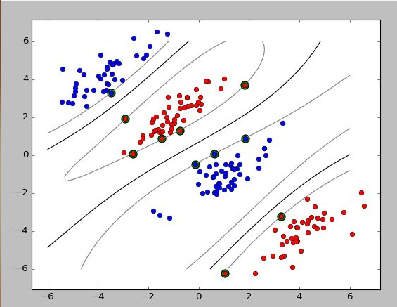
test_non_linear()
效果如下:
近期热文
加入微信机器学习交流群
请添加微信:guodongwe1991
备注姓名-单位-研究方向