R语言模拟:Bias Variance Decomposition

作者:量化小白一枚，上财研究生在读，偏向数据分析与量化投资

个人公众号:量化小白上分记 

接上一篇《R语言模拟：Bias-Variance trade-off》，本文通过模拟分析算法的泛化误差、偏差、方差和噪声之间的关系，是《element statistical learning》第七章的一个案例。

上一篇通过模拟给出了在均方误差度量下，测试集上存在的偏差方差Trade-Off的现象，随着模型复杂度（变量个数）增加，训练集上的误差不断减小，最终最终导致过拟合，而测试集的误差则先减小后增大。

模拟方法说明

本文通过对泛化误差的分解来说明训练集误差变化的原因，我们做如下模拟实验：

样本1：:训练集和测试集均为20个自变量，80个样本，自变量服从[0,1]均匀分布，因变量定义为：

Y = ifelse(X1>1/2,1,0)

样本2 ： 训练集和测试集均为20个自变量，80个样本，自变量服从[0,1]均匀分布，因变量定义为：

Y = ifelse(X1+X2+...+X10>5,1,0)

通过两类模型、两种误差度量方式共四种方法进行建模，分析误差，模型为knn和best subset linear model。 

knn根据距离样本最近的k个样本的Y值预测样本的Y值，knn模型用于样本1,R语言中可通过函数knnreg实现。

best subset linear model 对于输入的样本，获取最优的自变量组合建立线性模型进行预测，best subset model用于样本2，R语言中可通过函数regsubsets实现。

误差度量分为均方误差（squared error）和0-1误差（0-1 Loss）两种，均方误差可以视为回归模型（regression），0-1误差可以视为分类模型（classification）。

结果说明

每种方法模拟100次，在每个模型中计算偏差、方差和预测误差并作图分析结果，最终得到结果如下：

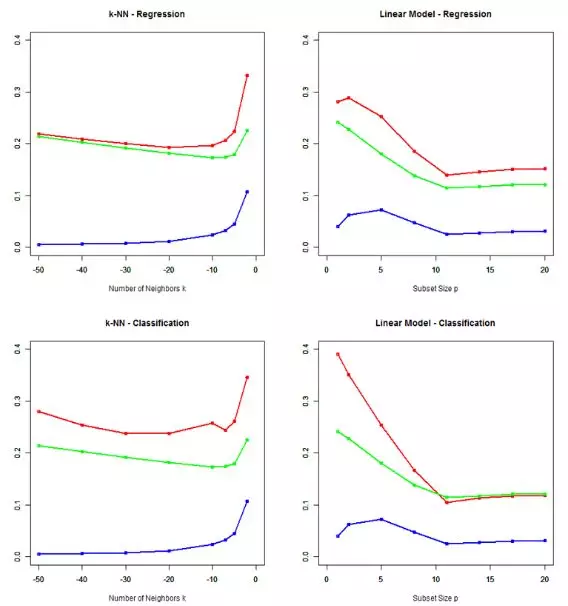
其中，红色线表示预测误差，蓝色线表示方差，绿色线表示偏差平方，对比书上的结果

结果分析：

1. 从数值上看，0-1 Loss 和Squared  error度量的模型具有不同特征，0-1 Loss满足预测误差 = 方差 +偏差平方的关系式，Squared error不满足这一关系；

2. 方差都是随着模型中包含变量个数增加而减小，偏差的变化非线性。

代码

语言：r

knn model

  1# bais variance trade-off  regression
  2
  3# knn 
  4
  5library(caret)
  6
  7# get bais variance
  8# k:knn中的k值或best subset中的k值
  9# num：模拟次数
 10# sigma:随机误差的标准差
 11# test_id 用于计算偏差误差的训练集样本编号，1-80中任一整数
 12# regtype:knn或best sub
 13# seeds:随机数种子
 14# 返回方差偏差误差等值
 15
 16getError <- function(k,num,modeltype,seeds,n_test){
 17  set.seed(seeds)
 18
 19
 20  testset <- as.data.frame(matrix(runif(n_test*21,0,1),n_test))
 21
 22  Allfx_hat <- matrix(0,n_test,num)
 23  Ally <- matrix(0,n_test,num)
 24  Allfx <- matrix(0,n_test,num)
 25
 26  # 模拟 num次 
 27
 28
 29
 30  for (i in 1:num){
 31    trainset <- as.data.frame(matrix(runif(80*21,0,1),80))
 32
 33
 34    fx_train <- ifelse(trainset[,1]>0.5,1,0)
 35    trainset[,21] <- fx_train
 36
 37    fx_test <- ifelse(testset[,1]>0.5,1,0)
 38    testset[,21] <- fx_test 
 39
 40
 41    # knn model
 42    knnmodel <- knnreg(trainset[,1:20],trainset[,21],k = k)
 43    probs <- predict(knnmodel, newdata = testset[,1:20])
 44
 45
 46    Allfx_hat[,i] <- probs
 47    Ally[,i] <- testset[,21]
 48    Allfx[,i] <- fx_test
 49
 50
 51
 52  } 
 53  # 计算方差、偏差等
 54
 55  # irreducible <- sigma^2
 56
 57  irreducible  <- mean(apply( Allfx - Ally  ,1,var))
 58  SquareBais  <- mean(apply((Allfx_hat - Allfx)^2,1,mean))
 59  Variance <- mean(apply(Allfx_hat,1,var))
 60
 61  # 回归或分类两种情况
 62  if (modeltype == 'reg'){
 63
 64    PredictError  <- irreducible + SquareBais + Variance 
 65
 66  }else{
 67
 68    PredictError  <- mean(ifelse(Allfx_hat>=0.5,1,0)!=Allfx)
 69  }
 70
 71
 72
 73  result <- data.frame(k,irreducible,SquareBais,Variance,PredictError)
 74
 75  return(result)
 76}
 77
 78# ----------------   plot square error  knn ----------------------------
 79
 80
 81
 82
 83# k:knn中的k值或best subset中的k值
 84# num：模拟次数
 85# test_id 用于计算偏差误差的训练集样本编号，1-80中任一整数
 86# regtype:knn或best sub
 87# seeds:随机数种子
 88
 89n_test <- 100
 90modeltype <- 'reg'
 91num <- 100
 92
 93seeds <- 1
 94
 95result <- getError(2,num,modeltype,seeds,n_test)
 96result <- rbind(result,getError(5,num,modeltype,seeds,n_test))
 97result <- rbind(result,getError(7,num,modeltype,seeds,n_test))
 98for (i in seq(10,50,10)){
 99  result <- rbind(result,getError(i,num,modeltype,seeds,n_test))
100
101}
102
103
104png(file = "k-NN - Regression_large_testset.png")
105
106plot(-result$k,result$PredictError,type = 'o',col = 'red',
107     xlim = c(-50,0),ylim = c(0,0.4),xlab = '', ylab ='', lwd = 2)
108par(new = T)
109plot(-result$k,result$SquareBais,type = 'o',col = 'green',
110     xlim = c(-50,0),ylim = c(0,0.4),xlab = '', ylab ='', lwd = 2)
111par(new = T) 
112plot(-result$k,result$Variance,type = 'o',col = 'blue',
113     xlim = c(-50,0),ylim = c(0,0.4),xlab = 'Number of Neighbors k', ylab ='', lwd = 2,
114     main = 'k-NN - Regression')
115dev.off()
116
117# ----------------------  plot 0-1 loss knn -------------------------
118modeltype <- 'classification'
119num <- 100
120n_test <- 100
121seeds <- 1
122
123result <- getError(2,num,modeltype,seeds,n_test)
124result <- rbind(result,getError(5,num,modeltype,seeds,n_test))
125result <- rbind(result,getError(7,num,modeltype,seeds,n_test))
126for (i in seq(10,50,10)){
127  result <- rbind(result,getError(i,num,modeltype,seeds,n_test))
128
129}
130
131
132png(file = "k-NN - Classification_large_testset.png")
133
134plot(-result$k,result$PredictError,type = 'o',col = 'red',
135     xlim = c(-50,0),ylim = c(0,0.4),xlab = '', ylab ='', lwd = 2)
136par(new = T)
137plot(-result$k,result$SquareBais,type = 'o',col = 'green',
138     xlim = c(-50,0),ylim = c(0,0.4),xlab = '', ylab ='', lwd = 2)
139par(new = T) 
140plot(-result$k,result$Variance,type = 'o',col = 'blue',
141     xlim = c(-50,0),ylim = c(0,0.4),xlab = 'Number of Neighbors k', ylab ='', lwd = 2,
142     main = 'k-NN - Classification')
143dev.off()

best subset model 

  1library(leaps) 
  2lm.BestSubSet<- function(trainset,k){
  3  lm.sub <- regsubsets(V21~.,trainset,nbest =1,nvmax = 20)
  4  summary(lm.sub)
  5  coef_lm <- coef(lm.sub,k)
  6  strings_coef_lm <- coef_lm
  7  x <- paste(names(coef_lm)[2:length(coef_lm)], collapse ='+')
  8  formulas <- as.formula(paste('V21~',x,collapse=''))
  9  return(formulas)
 10}
 11
 12getError <- function(k,num,modeltype,seeds,n_test){
 13  set.seed(seeds)
 14  testset <- as.data.frame(matrix(runif(n_test*21,0,1),n_test))
 15
 16  Allfx_hat <- matrix(0,n_test,num)
 17  Ally <- matrix(0,n_test,num)
 18  Allfx <- matrix(0,n_test,num)
 19
 20
 21  # 模拟 num次
 22
 23
 24
 25  for (i in 1:num){
 26    trainset <- as.data.frame(matrix(runif(80*21,0,1),80))
 27    fx_train <- ifelse(trainset[,1] +trainset[,2] +trainset[,3] +trainset[,4] +trainset[,5]+
 28                         trainset[,6] +trainset[,7] +trainset[,8] +trainset[,9] +trainset[,10]>5,1,0)
 29
 30    trainset[,21] <- fx_train
 31
 32    fx_test <- ifelse(testset[,1] +testset[,2] +testset[,3] +testset[,4] +testset[,5]+
 33                        testset[,6] +testset[,7] +testset[,8] +testset[,9] +testset[,10]>5,1,0)
 34
 35    testset[,21] <- fx_test 
 36
 37
 38    # best subset
 39    lm.sub <- lm(formula = lm.BestSubSet(trainset,k),trainset)
 40    probs <- predict(lm.sub,testset[,1:20], type = 'response')
 41
 42
 43    Allfx_hat[,i] <- probs
 44    Ally[,i] <- testset[,21]
 45    Allfx[,i] <- fx_test
 46
 47  } 
 48  # 计算方差、偏差等
 49
 50  # irreducible <- sigma^2
 51
 52  irreducible  <- mean(apply( Allfx - Ally  ,1,var))
 53  SquareBais  <- mean(apply((Allfx_hat - Allfx)^2,1,mean))
 54  Variance <- mean(apply(Allfx_hat,1,var))
 55
 56  # 回归或分类两种情况
 57  if (modeltype == 'reg'){
 58    PredictError <- irreducible + SquareBais + Variance 
 59  }else{
 60    PredictError <- mean(ifelse(Allfx_hat>=0.5,1,0)!=Allfx)
 61  }
 62  result <- data.frame(k,irreducible,SquareBais,Variance,PredictError)
 63  return(result)
 64}
 65
 66
 67
 68# ----------------   plot square error Best Subset Regression ----------------------------
 69
 70
 71modeltype <- 'reg'
 72num <- 100
 73n_test <- 1000
 74
 75seeds <- 4
 76all_p <- seq(2,20,3)
 77result <- getError(1,num,modeltype,seeds,n_test)
 78for (i in all_p){
 79  result <- rbind(result,getError(i,num,modeltype,seeds,n_test))
 80
 81}
 82
 83png(file = "Linear Model - Regression_large_testset.png")
 84
 85plot(result$k,result$PredictError,type = 'o',col = 'red',
 86     xlim = c(0,20),ylim = c(0,0.4),xlab = '', ylab ='', lwd = 2)
 87par(new = T)
 88plot(result$k,result$SquareBais,type = 'o',col = 'green',
 89     xlim = c(0,20),ylim = c(0,0.4),xlab = '', ylab ='', lwd = 2)
 90par(new = T) 
 91plot(result$k,result$Variance,type = 'o',col = 'blue',
 92     xlim = c(0,20),ylim = c(0,0.4),xlab = 'Subset Size p', ylab ='', lwd = 2,
 93     main = 'Linear Model - Regression')
 94dev.off()
 95
 96# ----------------------  plot 0-1 loss Best Subset Classification -------------------------
 97
 98modeltype <- 'classification'
 99num <- 100
100n_test <- 1000
101seeds <- 4
102
103
104all_p <- seq(2,20,3)
105result <- getError(1,num,modeltype,seeds,n_test)
106for (i in all_p){
107  result <- rbind(result,getError(i,num,modeltype,seeds,n_test))
108
109}
110
111png(file = "Linear Model - Classification_large_testset.png")
112
113
114plot(result$k,result$PredictError,type = 'o',col = 'red',
115     xlim = c(0,20),ylim = c(0,0.4),xlab = '', ylab ='', lwd = 2)
116par(new = T)
117plot(result$k,result$SquareBais,type = 'o',col = 'green',
118     xlim = c(0,20),ylim = c(0,0.4),xlab = '', ylab ='', lwd = 2)
119par(new = T) 
120plot(result$k,result$Variance,type = 'o',col = 'blue',
121     xlim = c(0,20),ylim = c(0,0.4),xlab = 'Subset Size p', ylab ='', lwd = 2,
122     main = 'Linear Model - Classification')
123# 
124dev.off()

参考文献

1. Ruppert D. The Elements of Statistical Learning: Data Mining, Inference, and Prediction[J]. Journal of the Royal Statistical Society, 2010, 99(466):567-567.

公众号后台回复关键字即可学习

回复 爬虫            爬虫三大案例实战  
回复 Python       1小时破冰入门

回复 数据挖掘     R语言入门及数据挖掘
回复 人工智能     三个月入门人工智能
回复 数据分析师  数据分析师成长之路 
回复 机器学习      机器学习的商业应用
回复 数据科学      数据科学实战
回复 常用算法      常用数据挖掘算法