八大直播作业-第五讲-Aringrhus

# coding: utf-8



# In[1]:





import numpy as np

import pandas as pd

from matplotlib import pyplot as plt

import statsmodels.api as sm

import statsmodels.formula.api as smf

import seaborn as sns

from scipy import stats

from sklearn.cross_validation import train_test_split

get_ipython().magic('matplotlib inline')





# In[2]:





telecom_churn = pd.read_csv(r'telecom_churn.csv')





# In[3]:





telecom_churn.head()

# In[4]:





cat_cols = ['churn','posTrend','negTrend','prom','curPlan','avgplan','planChange','posPlanChange','negPlanChange']

for col in cat_cols:

    telecom_churn[col] = telecom_churn[col].astype(int)

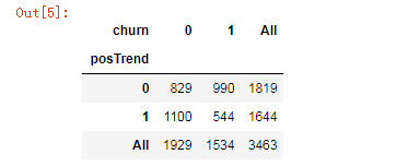
# # 两变量分析：检验该用户通话时长是否呈现出上升态势(posTrend)对流失(churn) 是否有预测价值



# In[5]:





cross1 = pd.crosstab(telecom_churn.posTrend,telecom_churn.churn, margins=True)

cross1

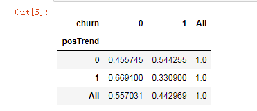
# In[6]:





def percConvert(ser):

    return ser/float(ser[-1])



cross1.apply(percConvert, axis=1)

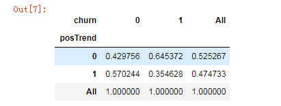
# In[7]:





cross1.apply(percConvert, axis=0)

# In[8]:





cross1.iloc[:2, :2]





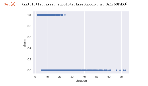
# In[9]:





telecom_churn.plot(x='duration', y='churn', kind='scatter')

# In[10]:





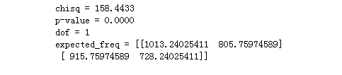
print('''chisq = %6.4f 

p-value = %6.4f

dof = %i 

expected_freq = %s'''  %stats.chi2_contingency(cross1.iloc[:2, :2]))

# # 首先将原始数据拆分为训练和测试数据集，使用训练数据集建立在网时长对流失的逻辑回归，使用测试数据集制作混淆矩阵（阈值为0.5），提供准确性、召回率指标，提供ROC曲线和AUC。



# In[11]:





X_train, X_test, y_train, y_test = train_test_split(telecom_churn.drop('churn',axis=1), telecom_churn['churn'], test_size=0.3, random_state=123)





# In[12]:





pd.concat([X_train,y_train],axis=1)





# In[13]:





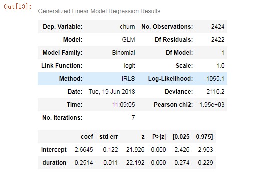
lg = smf.glm('churn ~ duration', data=pd.concat([X_train,y_train],axis=1), 

             family=sm.families.Binomial(sm.families.links.logit)).fit()

lg.summary()

# In[14]:





X_test.head(10)





# In[15]:





X_train['churn'] = y_train

X_test['proba'] = lg.predict(X_test)

X_train['proba'] = lg.predict(X_train.drop('churn',axis=1))

X_test['churn']= y_test

X_test.head(10)





# In[16]:





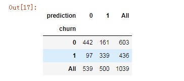
X_test['prediction'] = (X_test['proba'] > 0.5).astype('int')





# In[17]:





pd.crosstab(X_test.churn, X_test.prediction, margins=True)

# In[18]:





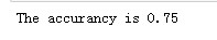
# 准确率

acc = sum(X_test['prediction'] == X_test['churn']) /np.float(len(X_test))

print('The accurancy is %.2f' %acc)

# In[19]:





X_test.loc[(X_test['prediction'] == 1) & (X_test['churn'] == 1)]





# In[20]:





# 召回率

recall = len(X_test[(X_test['prediction'] == 1) & (X_test['churn'] == 1)]) / sum(X_test['churn'] == 1)

print('The recall is %.2f' %recall)

# In[21]:





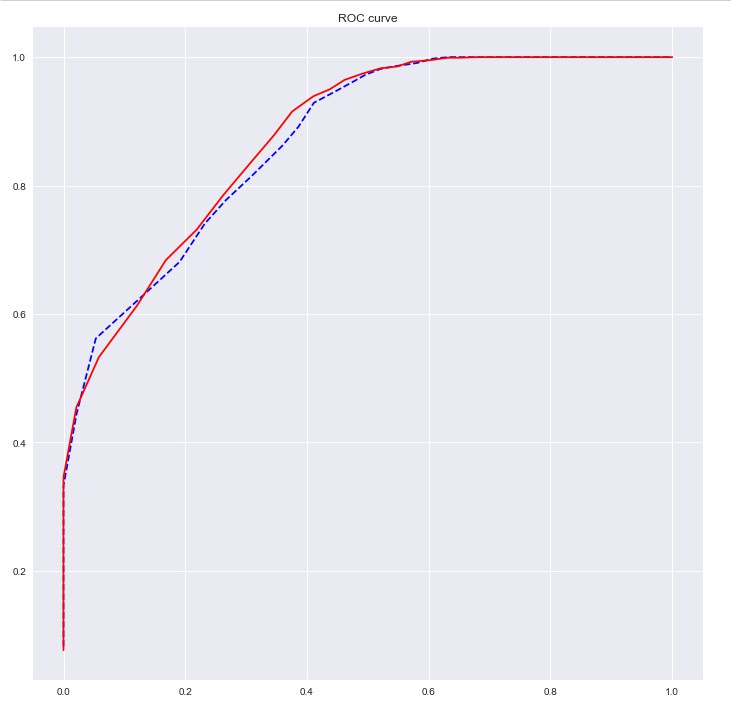
# ROC曲线



import sklearn.metrics as metrics



fpr_test, tpr_test, th_test = metrics.roc_curve(X_test.churn, X_test.proba)

fpr_train, tpr_train, th_train = metrics.roc_curve(X_train.churn, X_train.proba)



plt.figure(figsize=[12, 12])

plt.plot(fpr_test, tpr_test, 'b--')

plt.plot(fpr_train, tpr_train, '')

plt.title('ROC curve')

plt.show()

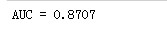
# In[22]:





print('AUC = %.4f' %metrics.auc(fpr_test, tpr_test))

# # 使用向前逐步法从其它备选变量中选择变量，构建基于AIC的最优模型，绘制ROC曲线，同时检验模型的膨胀系数



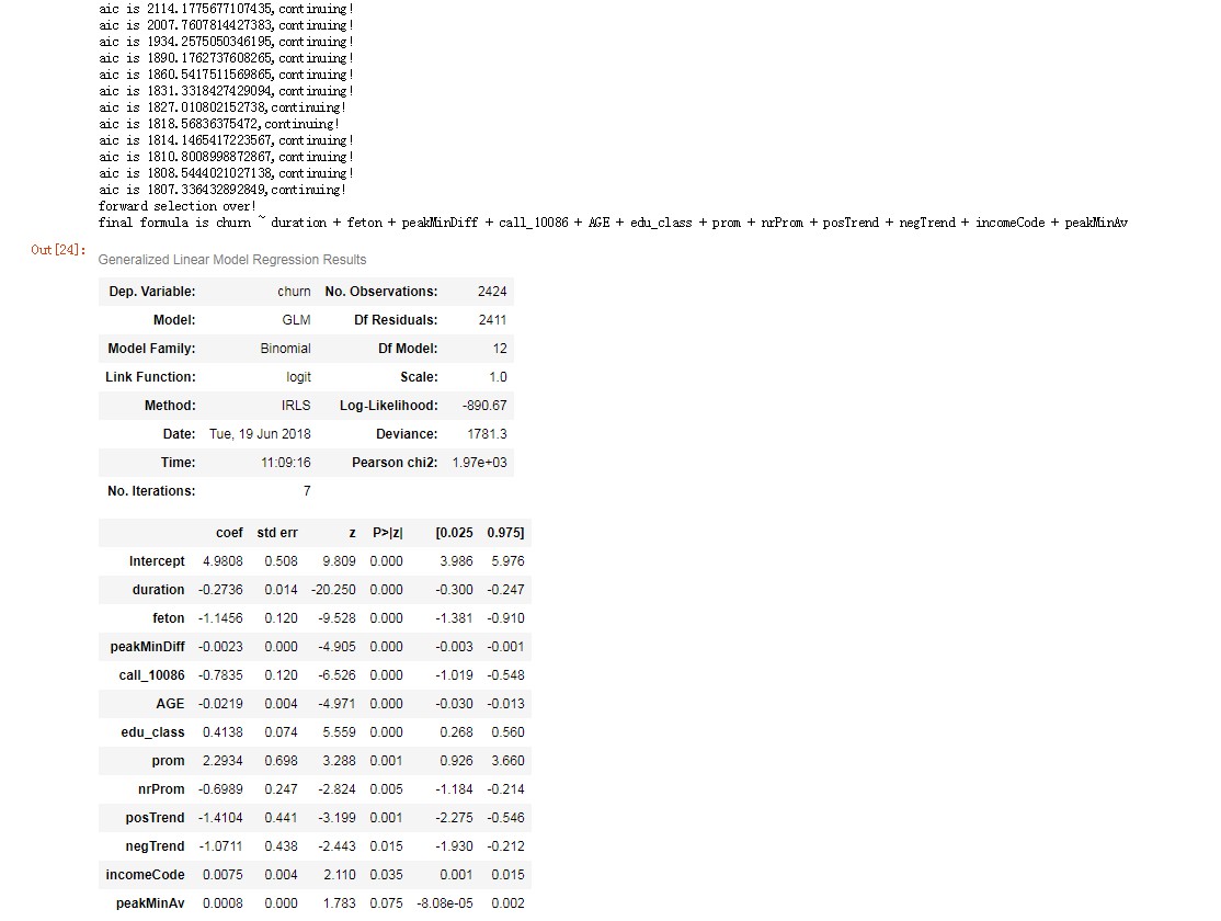
# In[23]:





# 向前法

def forward_select(data, response):

    remaining = set(data.columns)

    remaining.remove(response)

    selected = []

    current_score, best_new_score = float('inf'), float('inf')

    while remaining:

        aic_with_candidates=[]

        for candidate in remaining:

            formula = "{} ~ {}".format(

                response,' + '.join(selected + [candidate]))

            aic = smf.glm(

                formula=formula, data=data, 

                family=sm.families.Binomial(sm.families.links.logit)

            ).fit().aic

            aic_with_candidates.append((aic, candidate))

        aic_with_candidates.sort(reverse=True)

        best_new_score, best_candidate=aic_with_candidates.pop()

        if current_score > best_new_score: 

            remaining.remove(best_candidate)

            selected.append(best_candidate)

            current_score = best_new_score

            print ('aic is {},continuing!'.format(current_score))

        else:        

            print ('forward selection over!')

            break

            

    formula = "{} ~ {} ".format(response,' + '.join(selected))

    print('final formula is {}'.format(formula))

    model = smf.glm(

        formula=formula, data=data, 

        family=sm.families.Binomial(sm.families.links.logit)

    ).fit()

    return(model)

# In[24]:





candidates = ['churn','duration','AGE','edu_class','posTrend','negTrend','nrProm','prom','curPlan','avgplan','planChange','incomeCode','feton','peakMinAv','peakMinDiff','call_10086']

data_for_select = X_train[candidates]

lg_m1 = forward_select(data=data_for_select, response='churn')

lg_m1.summary()

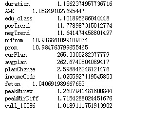
# In[25]:





def vif(df, col_i):

    from statsmodels.formula.api import ols

    

    cols = list(df.columns)

    cols.remove(col_i)

    cols_noti = cols

    formula = col_i + '~' + '+'.join(cols_noti)

    r2 = ols(formula, df).fit().rsquared

    return 1. / (1. - r2)

# In[26]:





exog = X_train[candidates].drop(['churn'], axis=1)

for i in exog.columns:

    print(i, '\t', vif(df=exog, col_i=i))

# In[27]:





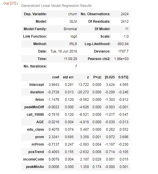
lg2 = smf.glm('churn ~ duration + feton + peakMinDiff + call_10086 + AGE + edu_class + prom + nrProm + posTrend  + incomeCode + peakMinAv', data=X_train.drop(['proba'],axis=1),

             family=sm.families.Binomial(sm.families.links.logit)).fit()

lg2.summary()

# In[28]:





# X_train.head()

X_test.head()





# In[29]:





X_train['proba2'] = lg2.predict(X_train.drop(['churn','proba'],axis=1))

X_test['proba2'] = lg2.predict(X_test.drop(['churn','proba','prediction'],axis=1))

print(X_train.head(10))

print(X_test.head(10))





# In[30]:





X_test['prediction2'] = (X_test['proba2'] > 0.5).astype('int')

# In[31]:





# 准确率

acc = sum(X_test['prediction2'] == X_test['churn']) /np.float(len(X_test))

print('The accurancy is %.2f' %acc)

# In[32]:





# 召回率

recall = len(X_test[(X_test['prediction2'] == 1) & (X_test['churn'] == 1)]) / sum(X_test['churn'] == 1)

print('The recall is %.2f' %recall)

# In[33]:





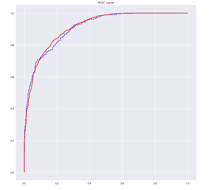
# ROC曲线



import sklearn.metrics as metrics



fpr_test, tpr_test, th_test = metrics.roc_curve(X_test.churn, X_test.proba2)

fpr_train, tpr_train, th_train = metrics.roc_curve(X_train.churn, X_train.proba2)



plt.figure(figsize=[12, 12])

plt.plot(fpr_test, tpr_test, 'b--')

plt.plot(fpr_train, tpr_train, '')

plt.title('ROC curve')

plt.show()

# In[34]:





print('AUC = %.4f' %metrics.auc(fpr_test, tpr_test))