shiny动态仪表盘应用——中国世界自然文化遗产可视化案例

这一篇很早就想写了，一直拖到现在都没写完。

虽然最近的社交网络上娱乐新闻热点特别多，想用来做可视化分析的素材简直多到不可想象，但是我个人一向不追星，对明星热文和娱乐类的新闻兴趣不是很大。还是更愿意把自己的精力贡献在那些不起眼的，然而却更能触动我们心灵与文化内涵的素材上来。

今天要写的主题中国的世界遗产名录，我将使用简单的网络数据抓取，多角度呈现我国当前已经拥有的世界遗产名录数目、类别、地域分布、详情介绍等。

http://www.zyzw.com/twzs010.htm

library("rvest")
library("stringr")
library("xlsx")

首先要确定好要爬取的目标信息。我感兴趣的是世界遗产的名称、申请成功的时间、分布的省份、遗产的性质、简介、详情页网址、预览图片地址。然后分析页面信息与后台代码，准备进入爬取阶段。

url<-"http://www.zyzw.com/twzs010.htm"
web<-read_html(url,encoding="GBK") 

Name<-web %>% html_nodes("b")%>%html_text(trim = FALSE)

%>%gsub("(\\n\\t|，|\\d|、)","",.)%>%grep("\\S",.,value=T)%>%str_trim(side="both")%>%.[1:54]

%>%.[setdiff(1:54,c(35,39))]

link<-paste0("http://www.zyzw.com/zgsjyc/zgsjyc",sprintf("d",1:52),".htm")

img_link<-paste0("http://www.zyzw.com/zgsjyc/zgsjyct/zgsjyc",sprintf("d",1:52),".jpg")

mydata<-data.frame(Name=Name,link=link,img_link)

write.xlsx(mydata,"E:/***/mydata.xlsx",sheetName="Sheet1",append=FALSE)

其他信息过于杂乱，抓取清洗非常耗时，索性手动在Excel里面清洗了。

setwd("E:/shiny/WorldHeritageSites")
library("xlsx")
library("lubridate")
library("ggplot2")
library("plyr")
library("RColorBrewer")
library("dplyr")
library("maptools")
library("ggthemes")
library("leafletCN")
library("leaflet")
library("htmltools")
library("shiny")
library("shinydashboard")
library("rgdal")

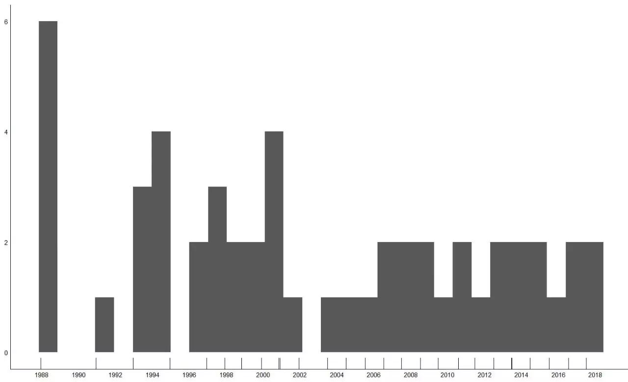
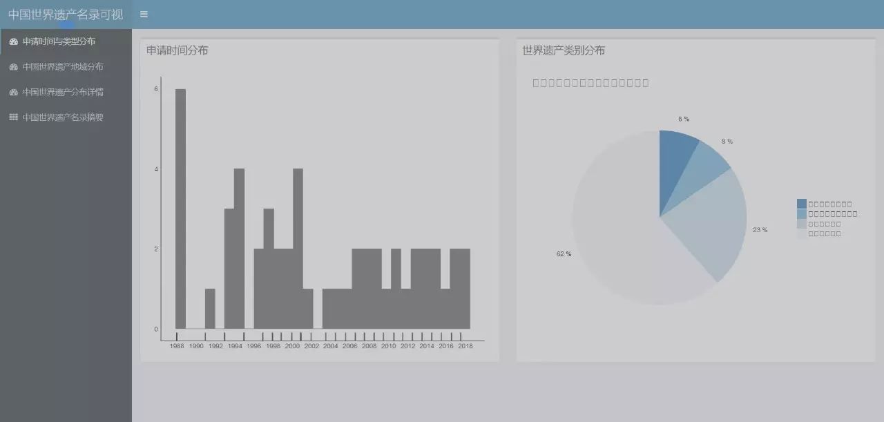
世界遗产申请年份频率统计：

mydata<-read.xlsx("./data/yichan.xlsx",sheetName="Sheet1",header=T,encoding='UTF-8',stringsAsFactors=FALSE,check.names=FALSE)



mydata$Time<-ymd(mydata$Time)

ggplot(mydata,aes(Time))+

geom_histogram(binh=30)+

geom_rug()+

scale_x_date(date_breaks="2 years",date_labels = "%Y")+

theme_void() %+replace%

theme(

     axis.text=element_text(),

     plot.margin = unit(c(1,1,1, 1), "lines"),

     axis.line=element_line()

   )

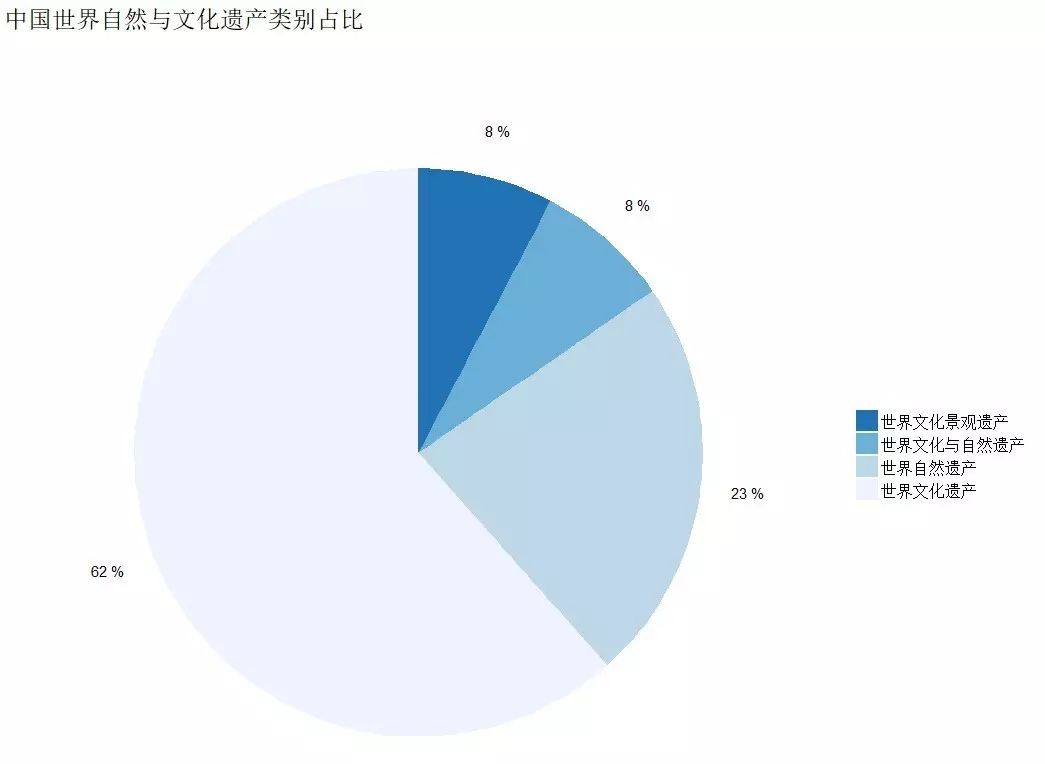
世界遗产类别统计：

class_count<-plyr::count(mydata$Class)

class_count<-arrange(class_count,freq)

class_count$label_y=c(0,cumsum(class_count$freq)[1:3])+class_count$freq/2class_count$x<-factor(class_count$x,levels=c("世界文化遗产","世界自然遗产","世界文化与自然遗产","世界文化景观遗产"),order=T)

ggplot(class_count,aes(x=1,y=freq,fill=x))+

geom_col()+

geom_text(aes(x=1.6,y=label_y,label=paste(round(class_count$freq*100/sum(class_count$freq)),"%")))+

coord_polar(theta="y")+

scale_fill_brewer()+

guides(fill=guide_legend(title=NULL,reverse=T))+

labs(title="中国世界自然与文化遗产类别占比")+

theme_void(base_size=15)%+replace%

theme(plot.margin = unit(c(1,1,1, 1), "lines"))

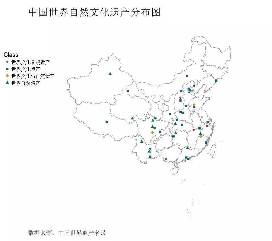
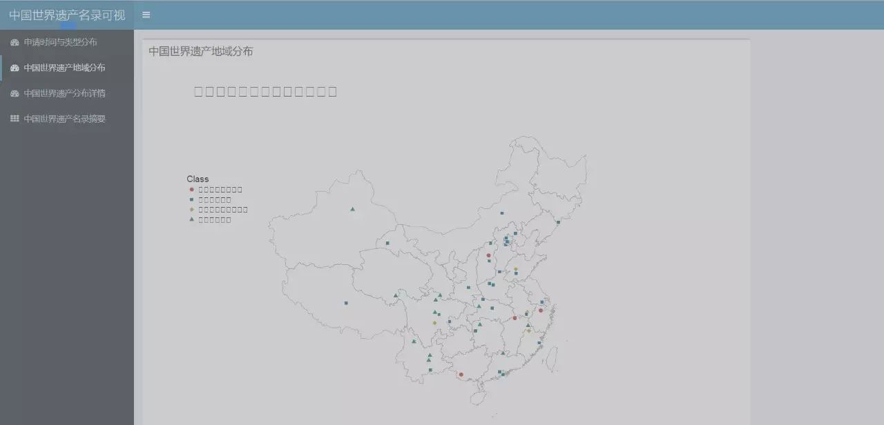
世界自然文化遗产地域分布：

china_map <- readOGR("D:/R/rstudy/CHN_adm/bou2_4p.shp",stringsAsFactors=FALSE)       

ggplot()+ 

geom_polygon(data=china_map,aes(x=long,y=lat,group=group),col="grey60",fill="white",size=.2,alpha=.4)+

geom_point(data=mydata,aes(x=long,y=lat,shape=Class,fill=Class),size=3,colour="white")+ 

     coord_map("polyconic") +

     scale_shape_manual(values=c(21,22,23,24))+

     scale_fill_wsj()+

     labs(title="中国世界自然文化遗产分布图",caption="数据来源：中国世界遗产名录")+   

     theme_void(base_size=15) %+replace%

     theme(

          plot.title=element_text(size=25,hjust=0),

          plot.caption=element_text(hjust=0),       

          legend.position = c(0.05,0.75),

          plot.margin = unit(c(1,0,1,0), "cm")

          )

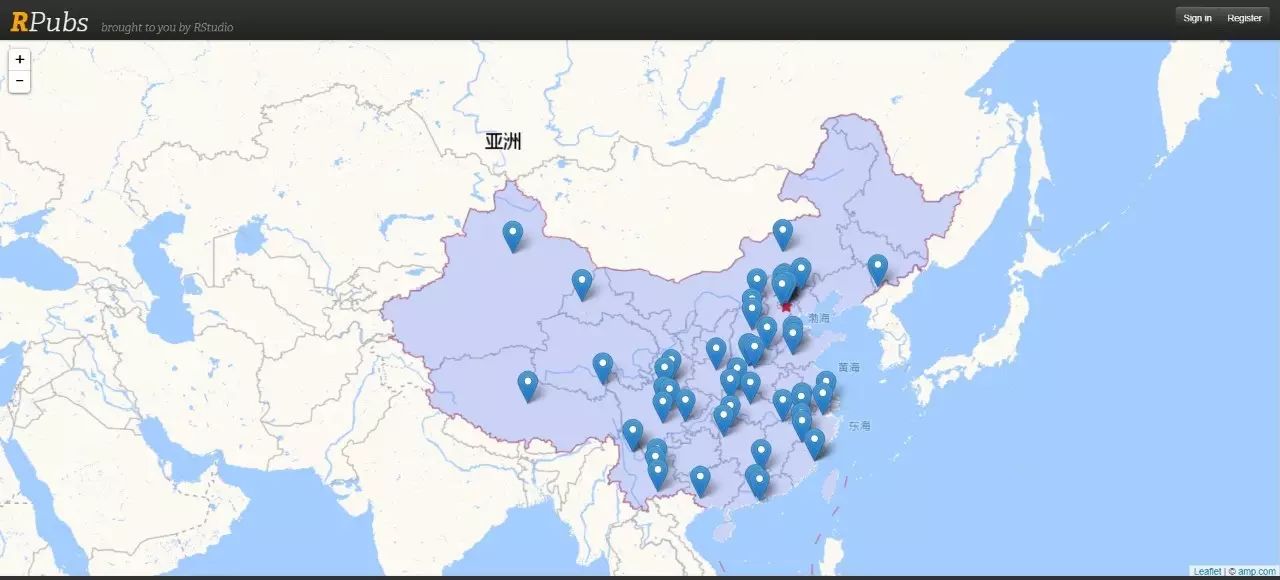
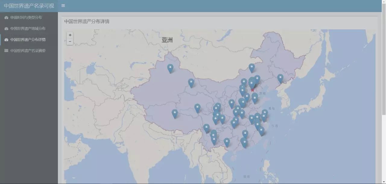
基于leaflet动态可视交互的世界自然文化遗产地理分布图

for(i in 1:nrow(mydata)){

     mydata$label[i]=sprintf(paste("<b><a href='https://ask.hellobi.com/%s'>%s</a></b>","<p>%s</p>","<p>%s</p>","<p><img src='%s' width='300'></p>",sep="<br/>"),

     mydata$link[i],mydata$Name[i],mydata$Class[i],mydata$Information[i],mydata$img_link[i])

}

leaflet(china_map)%>%amap()%>%addPolygons(stroke = FALSE)%>%

addMarkers(data=mydata,lng=~long,lat=~lat,popup=~label)

leaflet动态效果请点击这里：

http://rpubs.com/ljtyduyu/311149

接下来把以上所有代码封装成一个shinyAPP。

封装UI：

####封装UI：
ui <- dashboardPage(

  dashboardHeader(title = "中国世界遗产名录可视化"),

  dashboardSidebar(

    sidebarMenu(

      menuItem("申请时间与类型分布",     tabName = "dashboard1", icon = icon("dashboard")),

      menuItem("中国世界遗产地域分布",   tabName = "dashboard2", icon = icon("dashboard")),

      menuItem("中国世界遗产分布详情",   tabName = "dashboard3", icon = icon("dashboard")),

      menuItem("中国世界遗产名录摘要",   tabName = "widgets", icon = icon("th"))

    )

  ),



  dashboardBody(

    tabItems(



      tabItem(tabName = "dashboard1",

        fluidRow(

          box(

              title = "申请时间分布",

              plotOutput("plot1", height = 500)

          ),

          box(

              title = "世界遗产类别分布",

              plotOutput("plot2", height = 500)

          )

        )

      ),



      tabItem(tabName = "dashboard2",

      fluidRow(

          box(

              title = "中国世界遗产地域分布",

              plotOutput("plot3", width=1000, height=800),

              width =10

          )

        )

      ),



      tabItem(tabName = "dashboard3",

      fluidRow(

          box(

              title = "中国世界遗产分布详情",

              leafletOutput("plot4", width = "100%", height = 1000),

              width =12

          )

        )

      ),



      tabItem(tabName = "widgets",

      fluidRow(

          box(

              title = "中国世界遗产名录摘要",

              h4("中国作为著名的文明古国，自1985年加入世界遗产公约，至2017年7月，共有52个项目被联合国教科文组织列入《世界遗产名录》，与意大利并列世界第一。其中世界文化遗产32处，世界自然遗产12处，世界文化和自然遗产4处，世界文化景观遗产4处。源远流长的历史使中国继承了一份十分宝贵的世界文化和自然遗产，它们是人类的共同瑰宝。正一艺术最后编辑于2017年7月9日。"),width =12

          )

        )

      )



    )

  )

)

封装Server

server <- shinyServer(function(input, output) { 

  output$plot1 <- renderPlot({

           ggplot(mydata,aes(Time))+

           geom_histogram(binh=30)+

           geom_rug()+

           scale_x_date(date_breaks="2 years",date_labels = "%Y")+

           theme_void() %+replace%

           theme(axis.text=element_text(),plot.margin = unit(c(1,1,1, 1), "lines"),axis.line=element_line())

  })

  output$plot2 <- renderPlot({

        ggplot(class_count,aes(x=1,y=freq,fill=x))+

           geom_col()+

           geom_text(aes(x=1.6,y=label_y,label=paste(round(class_count$freq*100/sum(class_count$freq)),"%")))+

           coord_polar(theta="y")+

           scale_fill_brewer()+

           guides(fill=guide_legend(title=NULL,reverse=T))+

           labs(title="中国世界自然与文化遗产类别占比")+

           theme_void(base_size=15)%+replace%

           theme(plot.margin = unit(c(1,1,1,1), "lines"))

  })

  output$plot3 <- renderPlot({

           ggplot()+ 

           geom_polygon(data=china_map,aes(x=long,y=lat,group=group),col="grey60",fill="white",size=.2,alpha=.4)+

           geom_point(data=mydata,aes(x=long,y=lat,shape=Class,fill=Class),size=3,colour="white")+ 

           coord_map("polyconic") +

           scale_shape_manual(values=c(21,22,23,24))+

           scale_fill_wsj()+

           labs(title="中国世界自然文化遗产分布图",caption="数据来源：中国世界遗产名录")+   

           theme_void(base_size=15) %+replace%

           theme(

           plot.title=element_text(size=25,hjust=0),

           plot.caption=element_text(hjust=0),       

           legend.position = c(0.05,0.75),

           plot.margin = unit(c(1,0,1,0), "cm")

           )

  })

  output$plot4 <- renderLeaflet({

          leaflet(china_map)%>%amap()%>%addPolygons(stroke = FALSE)%>%

          addMarkers(data=mydata,lng=~long,lat=~lat,popup=~label)

  })

})

shinyApp(ui, server)

最终的web仪表盘预览效果：

在线课程请点击：https://edu.hellobi.com/course/195

数据源文件请移步本人GitHub：

https://github.com/ljtyduyu/DataWarehouse/tree/master/File