R_ggplot2地理信息可视化_史上最全（二）

作者：李誉辉  

四川大学在读研究生

前言

上文R_ggplot2地理信息可视化_史上最全（一）讲了sp和sf数据类型，这篇讲解地图数据集以及与其他几何对象的结合，还有栅格地图。

注：蓝字表示文末有其网址链接

4.地图数据集

地图数据集常见2中格式：

• json,包括GeoJSON(文件后缀为.geojson)和TopoJson(文件后缀为.json)。
  

• shp, shp对象比较特殊，是由很多个文件组成的，
  通常在同一个文件下还有.shx和.dbf格式的文件。这些文件必须在一起，否则不能成功读取。
  

• .rds,这是一种文件格式，分为sp.rds和sf.rds两种，分别对应p和sf两种数据结构。
  使用sp::readRDS()读取。

地图数据集读取包及函数

如上图所示,rgdal和sf功能比较全，用得也比较多。
地图集下载网站：

• GADM，注意该网站中，中国地图不包含台湾。
  

• 中国县级地图 （见文末）提取码：uomy
  

• OpenStreetMap
  

• 阿里云地图,左上角框框里面选择区域，左下角选择下载格式。

地图数据在线转换格式：

• geojson.io,在线解析和转换格式。
  

• mygeodata converter
  

• IGIS Map Converter

推荐使用rmapshaper::ms_simplify()简化地图数据，可以指定简化比例，不然真的很卡，
该包使用拓扑学的知识简化多边形，简化后在常规分辨率下根本看不出来差别。
该函数支持json，sp，sf等多种输入对象。
object.size()可以查看数据集的存储大小。

4.1 json格式

4.1.1 rgdal包读取

 1rm(list = ls()); gc() # 清空内存
 2library(ggplot2)
 3
 4path1 <- "E:/R_input_output/data_input/JSON/GeoJSON/China.geojson"
 5China_1 <- rgdal::readOGR(dsn = path1, stringsAsFactors = FALSE)
 6Encoding(China_1@data$name) <- "UTF-8" # 中文字符重编码
 7China_2 <- fortify(China_1)
 8
 9ggplot(China_2) + 
10  geom_polygon(aes(x = long, y = lat, group = group, fill = group), 
11               color = "cyan", show.legend = FALSE) + 
12  coord_map()

1##           used (Mb) gc trigger (Mb) max used (Mb)
2## Ncells  901585 48.2    1744096 93.2  1744096 93.2
3## Vcells 1789510 13.7    9804475 74.9 12236244 93.4
4## OGR data source with driver: GeoJSON 
5## Source: "E:\R_input_output\data_input\JSON\GeoJSON\China.geojson", layer: "中国"
6## with 35 features
7## It has 10 fields

4.2 sf包读取

sf包读取中文字符不会乱码。

 1rm(list = ls()); gc() # 清空内存
 2library(ggplot2)
 3library(sf)
 4
 5path1 <- "E:/R_input_output/data_input/JSON/GeoJSON/China.geojson"
 6China_1 <- st_read(path1, stringsAsFactors=FALSE)
 7
 8ggplot(China_1) + 
 9  geom_sf(color = "cyan", aes(fill = name), show.legend = FALSE) + 
10  coord_sf(crs = "+proj=aea +lat_1=25 +lat_2=50 +lon_0=105") + 
11  ggtitle("中国地图(Albers equal-area projection)")

 1##           used (Mb) gc trigger (Mb) max used (Mb)
 2## Ncells 1112615 59.5    1744096 93.2  1744096 93.2
 3## Vcells 2079841 15.9    9804475 74.9 12236244 93.4
 4## Reading layer `涓浗' from data source `E:\R_input_output\data_input\JSON\GeoJSON\China.geojson' using driver `GeoJSON'
 5## Simple feature collection with 35 features and 10 fields
 6## geometry type:  MULTIPOLYGON
 7## dimension:      XY
 8## bbox:           xmin: 73.50235 ymin: 3.397162 xmax: 135.0957 ymax: 53.56327
 9## epsg (SRID):    4326
10## proj4string:    +proj=longlat +datum=WGS84 +no_defs

4.3 shp格式

4.3.1 rgdal包读取

 1rm(list = ls()); gc() # 清空内存
 2library(ggplot2)
 3
 4path1 <- "E:/R_input_output/data_input/全国范围的行政边界和人口密度矢量图/CHN_adm/CHN_adm1.shp"
 5China_1 <- rgdal::readOGR(dsn = path1, stringsAsFactors = FALSE)
 6China_2 <- rmapshaper::ms_simplify(China_1) # 拓扑学知识简化数据
 7object.size(China_1); object.size(China_2) # 简化到不足1/10大小
 8
 9China_3 <- fortify(China_2) # 转变为sp对象的数据框,然后就没有@了
10ggplot(China_3) + 
11  geom_polygon(aes(x = long, y = lat, group = group,fill = group), 
12               color = "cyan", size = 0.5, show.legend = FALSE) + 
13  coord_map()

1##           used (Mb) gc trigger (Mb) max used (Mb)
2## Ncells 1113970 59.5    1744096 93.2  1744096 93.2
3## Vcells 2050141 15.7    9804475 74.9 12236244 93.4
4## OGR data source with driver: ESRI Shapefile 
5## Source: "E:\R_input_output\data_input\全国范围的行政边界和人口密度矢量图\CHN_adm\CHN_adm1.shp", layer: "CHN_adm1"
6## with 32 features
7## It has 16 fields
8## 17647616 bytes
9## 1590376 bytes

4.3.2 sf包读取

 1rm(list = ls()); gc() # 清空内存
 2library(ggplot2)
 3library(sf)
 4
 5path1 <- "E:/R_input_output/data_input/全国范围的行政边界和人口密度矢量图/CHN_adm/CHN_adm1.shp"
 6China_1 <- st_read(path1, stringsAsFactors=FALSE)
 7China_2 <- rmapshaper::ms_simplify(China_1) # 拓扑学知识简化数据
 8
 9ggplot(China_2) +
10  geom_sf(color = "cyan", aes(fill = NAME_1), show.legend = FALSE) + 
11  coord_sf(crs = "+proj=aea +lat_1=25 +lat_2=50 +lon_0=105") + 
12  ggtitle("中国大陆地图(Albers equal-area projection)")

 1##           used (Mb) gc trigger  (Mb) max used (Mb)
 2## Ncells 1349388 72.1    2132915 114.0  2132915  114
 3## Vcells 2990656 22.9   15829390 120.8 19786461  151
 4## Reading layer `CHN_adm1' from data source `E:\R_input_output\data_input\鍏ㄥ浗鑼冨洿鐨勮鏀胯竟鐣屽拰浜哄彛瀵嗗害鐭㈤噺鍥綷CHN_adm\CHN_adm1.shp' using driver `ESRI Shapefile'
 5## Simple feature collection with 32 features and 16 fields
 6## geometry type:  MULTIPOLYGON
 7## dimension:      XY
 8## bbox:           xmin: 73.5577 ymin: 15.78 xmax: 134.7739 ymax: 53.56086
 9## epsg (SRID):    4326
10## proj4string:    +proj=longlat +datum=WGS84 +no_defs

4.4 .rds数据格式

4.4.1 sp.rds数据

 1rm(list = ls()); gc() # 清空内存
 2library(ggplot2)
 3library(sp) # 使用readRDS函数读取.rds格式数据
 4
 5path2 <- "E:/R_input_output/data_input/gadm36_USA_1_sp.rds"
 6USA_1 <- readRDS(path2)
 7class(USA_1)
 8USA_2 <- rmapshaper::ms_simplify(USA_1) # 拓扑学知识简化数据
 9USA_3 <- fortify(USA_2) # 转化为sp对象的数据框
10
11ggplot(USA_3) + 
12  geom_polygon(aes(x = long, y = lat, group = group), 
13               fill = "lightpink", colour = "cyan", size = 0.5) + 
14  coord_map(xlim = c(-170, -60))

1##           used (Mb) gc trigger  (Mb) max used (Mb)
2## Ncells 1352847 72.3    2132915 114.0  2132915  114
3## Vcells 3317435 25.4   15829390 120.8 19786461  151
4## [1] "SpatialPolygonsDataFrame"
5## attr(,"package")
6## [1] "sp"

4.4.2 sf.rds数据

 1rm(list = ls()); gc() # 清空内存
 2library(ggplot2)
 3library(sp) # 使用readRDS函数读取.rds格式数据
 4
 5path2 <- "E:/R_input_output/data_input/gadm36_USA_1_sf.rds"
 6USA_1 <- readRDS(path2)
 7class(USA_1)
 8USA_2 <- rmapshaper::ms_simplify(USA_1) # 拓扑学知识简化数据
 9
10ggplot(USA_2) + 
11  geom_sf(aes(fill = NAME_1),colour = "cyan", size = 0.5, show.legend = FALSE) + 
12  coord_sf(xlim = c(-170, -60))

1##           used (Mb) gc trigger  (Mb) max used  (Mb)
2## Ncells 1353647 72.3    2710561 144.8  2710561 144.8
3## Vcells 4337426 33.1   33817672 258.1 42185982 321.9
4## [1] "sf"         "data.frame"

5.与其他几何对象结合

5.1 sp对象与其它几何对象结合

1rm(list = ls()); gc() # 清空内存
2library(ggplot2)

1##           used (Mb) gc trigger  (Mb) max used  (Mb)
2## Ncells 1359265 72.6    2710561 144.8  2710561 144.8
3## Vcells 4767536 36.4   26023171 198.6 42185982 321.9

5.1.1 气泡饼图

气泡饼图本来是可以用循环来绘制的。
但已经有现场的包了scatterpie。
里面有2个函数：

geom_scatterpie(), geom_scatterpie_legend()。
由于scatterpie目前不支持sf数据模型，
且下载的中国地图数据包经过fortify()转化后，与业务数据没有公共变量，
故不能合并数据集，只能用2个数据集绘图。

 1rm(list = ls()); gc() # 清空内存
 2library(ggplot2)
 3library(magrittr)
 4library(rgdal)
 5library(dplyr)
 6library(scatterpie)
 7
 8# 读取各省中心点坐标数据
 9path1 <- "E:/R_input_output/data_input/prov_centroids.csv"
10Prov_centers <- read.csv(path1, stringsAsFactors = FALSE)
11str(Prov_centers)
12
13# 读取地图坐标数据
14path2 <- "E:/R_input_output/data_input/JSON/GeoJSON/China.geojson"
15China_1 <- readOGR(path2, stringsAsFactors = FALSE)
16Encoding(China_1@data$name) <- "UTF-8" # 需要在fortify之前重编码
17China_1 <- fortify(China_1) # 
18
19# 编造业务数据
20n <- nrow(Prov_centers) # 34个省级行政单位
21set.seed(567)
22mydata_1 <- data.frame(
23  name = Prov_centers$name, 
24  radius = abs(rnorm(n, sd=2)),
25  A = abs(rnorm(n, sd=1)),
26  B = abs(rnorm(n, sd=2)),
27  C = abs(rnorm(n, sd=3)),
28  D = abs(rnorm(n, sd=4)),
29  stringsAsFactors = FALSE
30)
31mydata_1[1, 3:6] <- mydata_1[1, 3:6] * 3 # 更新第一行
32
33mydata_2 <- left_join(Prov_centers, mydata_1, by = "name") # 合并数据集
34
35
36ggplot(China_1) + 
37  geom_polygon(aes(x = long, y = lat, group = group), 
38               color = "black", fill=NA) + 
39  coord_map() + 
40  geom_scatterpie(data = mydata_2,
41                  aes(x = x, y = y, group = name, r = radius/1.5), # 只能在此更改标度
42                  cols = LETTERS[1:4], color = NA, alpha = 0.5) + 
43  geom_scatterpie_legend(mydata_2$radius, x = 130, y = 15)  # 半径图例起点坐标
44

 1##           used (Mb) gc trigger  (Mb) max used  (Mb)
 2## Ncells 1359664 72.7    2710561 144.8  2710561 144.8
 3## Vcells 4770797 36.4   20818536 158.9 42185982 321.9
 4## 'data.frame':    34 obs. of  4 variables:
 5##  $ id_numbers: int  1 2 3 4 5 6 7 8 9 10 ...
 6##  $ x         : num  85.2 88.4 113.9 96 102.7 ...
 7##  $ y         : num  41.1 31.5 44.1 35.7 30.6 ...
 8##  $ name      : chr  "新疆维吾尔自治区" "西藏自治区" "内蒙古自治区" "青海省" ...
 9## OGR data source with driver: GeoJSON 
10## Source: "E:\R_input_output\data_input\JSON\GeoJSON\China.geojson", layer: "中国"
11## with 35 features
12## It has 10 fields

5.2 sf对象与其它几何对象结合

5.2.1 插入散点图

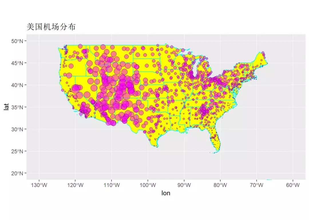
我们使用的数据来自nycflights13数据包。一个美国民航领域的数据包。
其内含有5个数据集：flights, weather, planes, airports, airlines。

散点图一般坐标列的长度与地图数据集坐标列长度不一样，所以通常在ggplot2中用2个数据集绘图。
首先传递地图数据集，
在散点图的时候，指定新的数据集。
根据图层叠加原理，后添加的图层在表层。
最后进行坐标变换。
这里有个bug,变换为某些地图投影后，叠加的几何对象图层就消失了，只剩地图底层了。

 1rm(list = ls()); gc() # 清空内存
 2library(ggplot2)
 3library(nycflights13) 
 4
 5class(airports)
 6
 7path1 <- "E:/R_input_output/data_input/cb_2013_us_state_20m/cb_2013_us_state_20m.shp"
 8USA_cencus <- sf::st_read(dsn = path1)
 9
10ggplot(USA_cencus) +
11  geom_sf(fill = "yellow", color = "cyan") +
12  geom_point(data = airports, # 更改数据源，点的数据与地图底层不一样
13             aes(x = lon, y = lat, size = alt), 
14             shape = 21, fill = "magenta", alpha = 0.5) + 
15  coord_sf(xlim = c(-130, -60), ylim = c(20, 50)) + # 设定显示范围
16  scale_size_area(guide = FALSE) + 
17  ggtitle("美国机场分布") # 指定标题
18

 1##           used (Mb) gc trigger  (Mb) max used  (Mb)
 2## Ncells 1418752 75.8    2710561 144.8  2710561 144.8
 3## Vcells 4685554 35.8   20818536 158.9 42185982 321.9
 4## [1] "tbl_df"     "tbl"        "data.frame"
 5## Reading layer `cb_2013_us_state_20m' from data source `E:\R_input_output\data_input\cb_2013_us_state_20m\cb_2013_us_state_20m.shp' using driver `ESRI Shapefile'
 6## Simple feature collection with 52 features and 9 fields
 7## geometry type:  MULTIPOLYGON
 8## dimension:      XY
 9## bbox:           xmin: -179.1473 ymin: 17.88481 xmax: 179.7785 ymax: 71.35256
10## epsg (SRID):    4269
11## proj4string:    +proj=longlat +datum=NAD83 +no_defs

5.2.2 插入气泡图

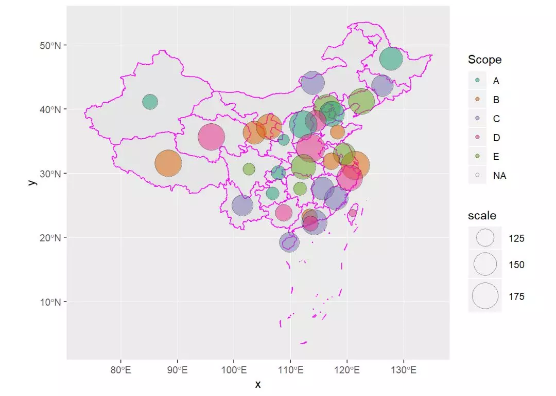
很多时候，我们需要每个行政区一个图。
这时候可以合并数据集。
将业务数据与行政区域地图数据合并。然后绘图。

中国各省中心点坐标数据（见文末）提取码：kj2a。

 1rm(list = ls()); gc() # 清空内存
 2library(ggplot2)
 3library(sf)
 4library(magrittr)
 5library(rgdal)
 6library(dplyr)
 7
 8# 读取各省中心点坐标数据
 9path1 <- "E:/R_input_output/data_input/prov_centroids.csv"
10Prov_centers <- read.csv(path1, stringsAsFactors = FALSE)
11str(Prov_centers)
12
13# 读取地图坐标数据
14path2 <- "E:/R_input_output/data_input/JSON/GeoJSON/China.geojson"
15China_1 <- st_read(path2, stringsAsFactors=FALSE)
16
17# 编造业务数据
18mydata_1 <- data.frame(
19  id = 1:34,
20  name = Prov_centers$name,
21  scale = runif(34,100,200) %>% round(),
22  Scope = rep(LETTERS[1:5],length = 34)
23)
24
25# 合并数据集
26mydata_2 <- left_join(Prov_centers, mydata_1, by = "name")
27mydata_3 <- left_join(China_1, mydata_2, by = "name")
28
29# 在地图上绘制气泡图
30ggplot(mydata_3) + 
31  geom_sf(color = "magenta") +
32  geom_point(aes(x = x, y = y, fill = Scope, size = scale),
33             shape = 21, alpha = 0.5) + 
34  coord_sf() + # 
35  scale_fill_brewer(palette = "Dark2") + 
36  scale_size(range = c(3, 12))

 1##           used (Mb) gc trigger  (Mb) max used  (Mb)
 2## Ncells 1424971 76.2    2710561 144.8  2710561 144.8
 3## Vcells 4745575 36.3   20818536 158.9 42185982 321.9
 4## 'data.frame':    34 obs. of  4 variables:
 5##  $ id_numbers: int  1 2 3 4 5 6 7 8 9 10 ...
 6##  $ x         : num  85.2 88.4 113.9 96 102.7 ...
 7##  $ y         : num  41.1 31.5 44.1 35.7 30.6 ...
 8##  $ name      : chr  "新疆维吾尔自治区" "西藏自治区" "内蒙古自治区" "青海省" ...
 9## Reading layer `涓浗' from data source `E:\R_input_output\data_input\JSON\GeoJSON\China.geojson' using driver `GeoJSON'
10## Simple feature collection with 35 features and 10 fields
11## geometry type:  MULTIPOLYGON
12## dimension:      XY
13## bbox:           xmin: 73.50235 ymin: 3.397162 xmax: 135.0957 ymax: 53.56327
14## epsg (SRID):    4326
15## proj4string:    +proj=longlat +datum=WGS84 +no_defs

5.2.3 填充颜色

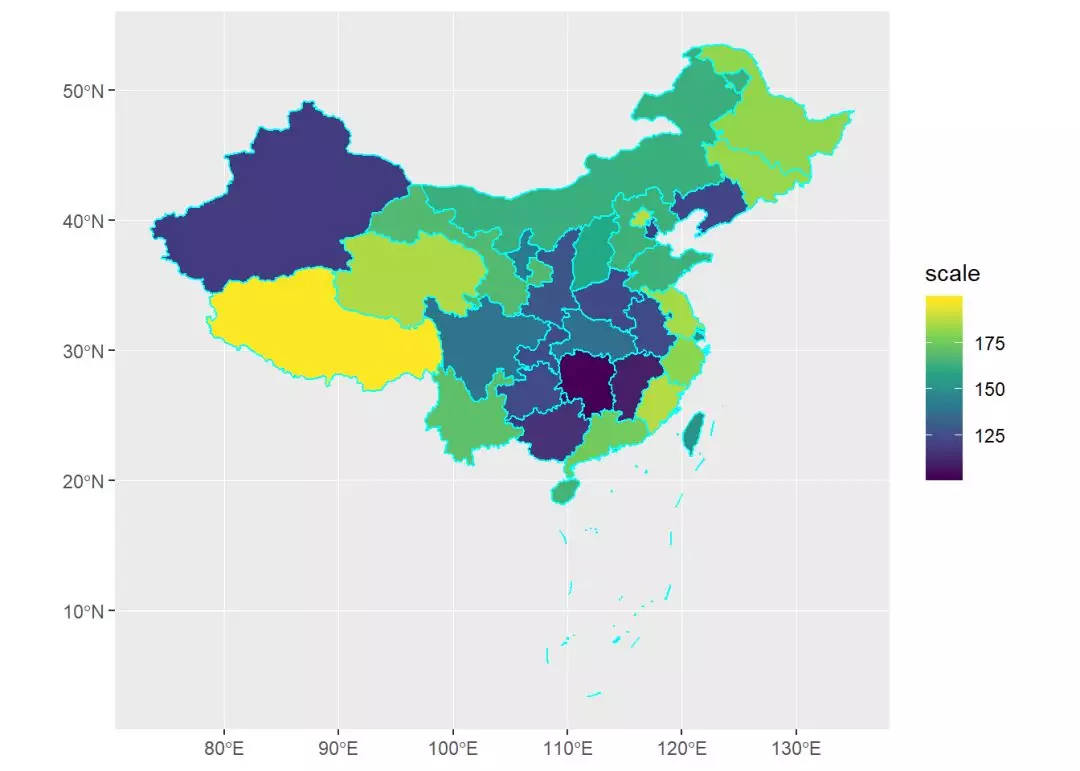
基于变量给行政区域填充颜色。

 1rm(list = ls()); gc() # 清空内存
 2library(ggplot2)
 3
 4rm(list = ls()); gc() # 清空内存
 5library(ggplot2)
 6library(sf)
 7library(magrittr)
 8library(rgdal)
 9library(dplyr)
10
11# 读取各省中心点坐标数据
12path1 <- "E:/R_input_output/data_input/prov_centroids.csv"
13Prov_centers <- read.csv(path1, stringsAsFactors = FALSE)
14str(Prov_centers)
15
16# 读取地图坐标数据
17path2 <- "E:/R_input_output/data_input/JSON/GeoJSON/China.geojson"
18China_1 <- st_read(path2, stringsAsFactors=FALSE)
19
20# 编造业务数据
21mydata_1 <- data.frame(
22  id = 1:34,
23  name = Prov_centers$name,
24  scale = runif(34,100,200) %>% round(),
25  Scope = rep(LETTERS[1:5],length = 34)
26)
27
28# 合并数据集
29mydata_2 <- left_join(Prov_centers, mydata_1, by = "name")
30mydata_3 <- left_join(China_1, mydata_2, by = "name")
31
32# 连续变量
33ggplot(mydata_3) + 
34  geom_sf(aes(fill = scale), color = "cyan") +
35  coord_sf() + 
36  scale_fill_continuous(type = "viridis") # 调整颜色标度
37
38# 离散变量
39ggplot(mydata_3) + 
40  geom_sf(aes(fill = Scope), color = "cyan") +
41  coord_sf() + 
42  scale_fill_brewer(palette = "Dark2") # 调整颜色标度

 1##           used (Mb) gc trigger  (Mb) max used  (Mb)
 2## Ncells 1425301 76.2    2710561 144.8  2710561 144.8
 3## Vcells 4676860 35.7   20818536 158.9 42185982 321.9
 4##           used (Mb) gc trigger  (Mb) max used  (Mb)
 5## Ncells 1425323 76.2    2710561 144.8  2710561 144.8
 6## Vcells 4676895 35.7   20818536 158.9 42185982 321.9
 7## 'data.frame':    34 obs. of  4 variables:
 8##  $ id_numbers: int  1 2 3 4 5 6 7 8 9 10 ...
 9##  $ x         : num  85.2 88.4 113.9 96 102.7 ...
10##  $ y         : num  41.1 31.5 44.1 35.7 30.6 ...
11##  $ name      : chr  "新疆维吾尔自治区" "西藏自治区" "内蒙古自治区" "青海省" ...
12## Reading layer `涓浗' from data source `E:\R_input_output\data_input\JSON\GeoJSON\China.geojson' using driver `GeoJSON'
13## Simple feature collection with 35 features and 10 fields
14## geometry type:  MULTIPOLYGON
15## dimension:      XY
16## bbox:           xmin: 73.50235 ymin: 3.397162 xmax: 135.0957 ymax: 53.56327
17## epsg (SRID):    4326
18## proj4string:    +proj=longlat +datum=WGS84 +no_defs

5.2.4 插入条形图

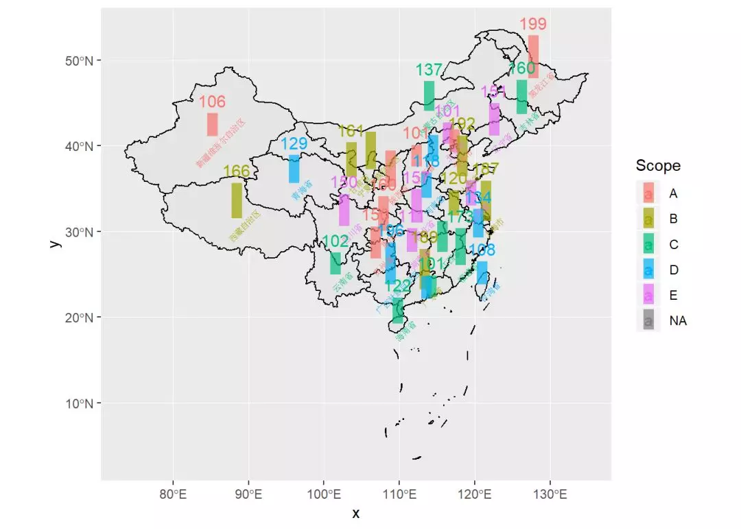
因为geom_bar()或geom_col()绘制柱形图，其y坐标代表柱子的高度，而不是纬度。
所有不能之间使用其绘制条形图。
这里使用geom_linerange()函数插入柱形图。
geom_linerange()内有多个映射参数包括：x,ymin, ymax, size。

 1rm(list = ls()); gc() # 清空内存
 2library(ggplot2)
 3
 4rm(list = ls()); gc() # 清空内存
 5library(ggplot2)
 6library(sf)
 7library(magrittr)
 8library(rgdal)
 9library(dplyr)
10
11# 读取各省中心点坐标数据
12path1 <- "E:/R_input_output/data_input/prov_centroids.csv"
13Prov_centers <- read.csv(path1, stringsAsFactors = FALSE)
14str(Prov_centers)
15
16# 读取地图坐标数据
17path2 <- "E:/R_input_output/data_input/JSON/GeoJSON/China.geojson"
18China_1 <- st_read(path2, stringsAsFactors=FALSE)
19
20# 编造业务数据
21mydata_1 <- data.frame(
22  id = 1:34,
23  name = Prov_centers$name,
24  scale = runif(34,100,200) %>% round(),
25  Scope = rep(LETTERS[1:5],length = 34)
26)
27
28# 合并数据集
29mydata_2 <- left_join(Prov_centers, mydata_1, by = "name")
30mydata_3 <- left_join(China_1, mydata_2, by = "name")
31
32# 绘制条形图
33ggplot(mydata_3) + 
34  geom_sf(color = "black") +
35  geom_linerange(aes(x = x, ymin = y, ymax = y + scale/40, color = Scope),
36           alpha = 0.7, size = 3.5) + 
37  geom_text(aes(x = x, y = y, label = name, color = Scope), # 添加行政区域名称
38            size = 2, vjust = 2, angle = 45, check_overlap = TRUE) + 
39  geom_text(aes(x = x, y = y + scale/40, label = scale, color = Scope), # 添加数字标签
40            size = 4, vjust = -0.5, check_overlap = TRUE) + 
41  coord_sf() + 
42  scale_fill_brewer(palette = "Dark2") # 调整颜色标度
43

 1##           used (Mb) gc trigger  (Mb) max used  (Mb)
 2## Ncells 1432071 76.5    2710561 144.8  2710561 144.8
 3## Vcells 4697138 35.9   20818536 158.9 42185982 321.9
 4##           used (Mb) gc trigger  (Mb) max used  (Mb)
 5## Ncells 1432090 76.5    2710561 144.8  2710561 144.8
 6## Vcells 4697168 35.9   20818536 158.9 42185982 321.9
 7## 'data.frame':    34 obs. of  4 variables:
 8##  $ id_numbers: int  1 2 3 4 5 6 7 8 9 10 ...
 9##  $ x         : num  85.2 88.4 113.9 96 102.7 ...
10##  $ y         : num  41.1 31.5 44.1 35.7 30.6 ...
11##  $ name      : chr  "新疆维吾尔自治区" "西藏自治区" "内蒙古自治区" "青海省" ...
12## Reading layer `涓浗' from data source `E:\R_input_output\data_input\JSON\GeoJSON\China.geojson' using driver `GeoJSON'
13## Simple feature collection with 35 features and 10 fields
14## geometry type:  MULTIPOLYGON
15## dimension:      XY
16## bbox:           xmin: 73.50235 ymin: 3.397162 xmax: 135.0957 ymax: 53.56327
17## epsg (SRID):    4326
18## proj4string:    +proj=longlat +datum=WGS84 +no_defs

6.栅格地图

栅格数据可以映射到地图上，但是很多时候变量通常是点数据，如各个气象观测点的气象数据。
这时候需要用插值将点数据插值成栅格数据，再添加到地图底图上。
ggplot2这个实现该功能比较困难。geom_raster()及stat_density_2d()只能使用栅格数据。
这里推荐使用tmap包实现栅格颜色可视化地图。

7.参考资料

geom_map

https://ggplot2.tidyverse.org/reference/geom_map.html

coord_map

https://ggplot2.tidyverse.org/reference/coord_map.html

geom_density_2d

https://ggplot2.tidyverse.org/reference/geom_density_2d.html

geom_tile

https://ggplot2.tidyverse.org/reference/geom_tile.html

利用R语言绘制世界航班路线图

scatterpie离散饼图

https://cran.r-project.org/web/packages/scatterpie/vignettes/scatterpie.html

ggplot2与sf包结合画地图

https://cfss.uchicago.edu/geoviz_plot.html

部分地图投影参考图

https://www.r-bloggers.com/map-projections-in-oce/

Projectionlist源码

https://github.com/zachcp/phylogeo/blob/master/R/utility-functions.R

sf对象详细介绍

https://cran.r-project.org/web/packages/sf/vignettes/sf1.html#what_is_a_feature

rgdal Tips

http://zevross.com/blog/2016/01/13/tips-for-reading-spatial-files-into-r-with-rgdal/

手把手教你使用ggplot2绘制中国地图

weather Visualizatio

https://homepage.divms.uiowa.edu/~luke/classes/STAT4580/weather.html

文中网址

墨卡托投影 

http://desktop.arcgis.com/zh-cn/arcmap/10.3/guide-books/map-projections/mercator.htm

正弦曲线投影

http://desktop.arcgis.com/zh-cn/arcmap/10.3/guide-books/map-projections/sinusoidal.htm

摩尔维特投影

http://desktop.arcgis.com/zh-cn/arcmap/10.3/guide-books/map-projections/mollweide.htm

等距方位投影

http://desktop.arcgis.com/zh-cn/arcmap/10.3/guide-books/map-projections/azimuthal-equidistant.htm

亚尔勃斯等积圆锥投影

http://desktop.arcgis.com/zh-cn/arcmap/10.3/guide-books/map-projections/albers-equal-area-conic.htm

球心投影

http://desktop.arcgis.com/zh-cn/arcmap/10.3/guide-books/map-projections/gnomonic.htm

正射投影

http://desktop.arcgis.com/zh-cn/arcmap/10.3/guide-books/map-projections/orthographic.htm

简单圆锥投影

http://desktop.arcgis.com/zh-cn/arcmap/10.3/guide-books/map-projections/simple-conic.htm

兰勃特等角圆锥投影

http://desktop.arcgis.com/zh-cn/arcmap/10.3/guide-books/map-projections/lambert-conformal-conic.htm

Projection methods

https://proj4.org/operations/projections/index.html

GADM

https://gadm.org/download_country_v3.html

中国县级地图 

https://pan.baidu.com/share/init?surl=JALgWfl7CmlntmujyqtjaQ 提取码：uomy

OpenStreetMap

https://www.openstreetmap.org./#map=1/-70/111

阿里云地图,

http://datav.aliyun.com/tools/atlas/#&lat=33.521903996156105&lng=104.29849999999999&zoom=4

geojson.io

http://geojson.io/#map=7/36.421/118.751

mygeodata converter

https://mygeodata.cloud/converter/shp-to-geojson

IGIS Map Converter

https://map.igismap.com/converter

中国各省中心点坐标数据

https://pan.baidu.com/share/init?surl=tFK7HBjpWF3cJ9M4rJgVZA

 提取码：kj2a

往期精彩：

• R_插值_拟合_回归_样条

• R_circlize包_和弦图（一）

• R_ggplot2基础（一）

• R_3D图(一)