
作者:黄天元,复旦大学博士在读,目前研究涉及文本挖掘、社交网络分析和机器学习等。希望与大家分享学习经验,推广并加深R语言在业界的应用。
邮箱:huang.tian-yuan@qq.com
经常玩数据竞赛的人几乎达成了一个共识,就是建模过程大家都大同小异,但是特征工程则至关重要。数据和特征决定了机器学习的上限,而模型和算法只是逼近这个上限而已。这里将会介绍一些最基本的特征工程方法以及代码的实现,供大家参考。这次的数据可以在下面网站找到:https://github.com/dipanjanS/practical-machine-learning-with-python/tree/master/notebooks/Ch04_Feature_Engineering_and_Selection/datasets
Python
基本设置
#加载包
import pandas as pd

import matplotlib.pyplot as plt

import matplotlib as mpl

import numpy as np

import scipy.stats as spstats

#对图像输出的统一设置

%matplotlib inline

mpl.style.reload_library()

mpl.style.use('classic')

mpl.rcParams['figure.facecolor'] = (1, 1, 1, 0)

mpl.rcParams['figure.figsize'] = [6.0, 4.0]

mpl.rcParams['figure.dpi'] = 100

file_path = "G:/Py/practical-machine-learning-with-python-master/notebooks/Ch04_Feature_Engineering_and_Selection/"原始数据特征
看到这份数据介绍的时候我也是惊呆了,这是关于“口袋妖怪”游戏的一个数据集,上面是关于一些妖怪们的攻击力、防御力、生命值、速度之类的参数,这个动画在我那个年代叫做“宠物小精灵”...Anyway,我们这个例子要看的就是数值型变量的基本特征,我们选其中三个进行观察。
poke_df = pd.read_csv(file_path + 'datasets/Pokemon.csv',

                      encoding='utf-8')

poke_df.head()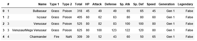
poke_df[['HP', 'Attack', 'Defense']].head()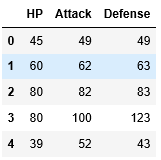
poke_df[['HP', 'Attack', 'Defense']].describe()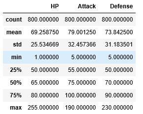
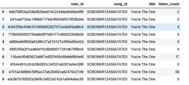
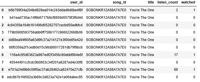
另外,有的原始数值型变量是通过计数来表示的,比如下面例子是用户听歌的记录,其中listen_count记录的是用户听了一首歌多少次。
popsong_df = pd.read_csv(file_path + 'datasets/song_views.csv', encoding='utf-8')

popsong_df.head(10)
二值化
关于听歌的案例,其实有一种粗略的理解,就是听过还是没听过,也就是不管听了多少次,只要不是没听过,就记录为1,其他是0.对于一些问题来说,听歌的绝对次数其实并不重要,比如一首歌的用户覆盖面,就不需要考虑哪些用户特别喜欢这首歌的问题。
#提取用户是否听过这首歌的特征

watched = np.array(popsong_df['listen_count'])

watched[watched >= 1] = 1

popsong_df['watched'] = watched

popsong_df.head(10)
#sklearn用专门的函数来完成这个任务

from sklearn.preprocessing import Binarizer

bn = Binarizer(threshold=0.9)

pd_watched = bn.transform([popsong_df['listen_count']])[0]

popsong_df['pd_watched'] = pd_watched

popsong_df.head(11)
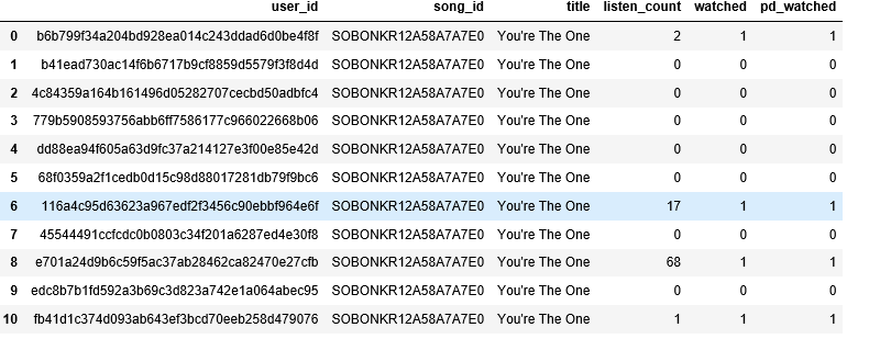
Binarizer函数的阈值设定含义为,小于等于阈值的值都视为0,大于阈值的则视为1.
取整
有时候数据真的不需要太高的精度,高精度的数据会占用更多的内存,因此可以取整处理。应该说这种操作肯定是会损失信息量的,但是如果在一些情况下5.9和6.3被认为没有差别的时候,取整也许更加合适。
items_popularity = pd.read_csv(file_path + 'datasets/item_popularity.csv', encoding='utf-8')

items_popularity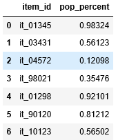
这个例子中,pop_percent的数据是百分比,因此我们可以用几成或百分点为单位来表示。
items_popularity['popularity_scale_10'] = np.array(np.round((items_popularity['pop_percent'] * 10)), dtype='int')

items_popularity['popularity_scale_100'] = np.array(np.round((items_popularity['pop_percent'] * 100)), dtype='int')

items_popularity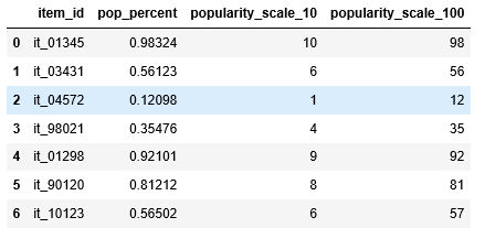
交互项构造
如果认为一些变量的平方项更有可能与因变量成一定关系,就应该构造二次项甚至是更高次的交互项。比如,我们如果有草地的长宽,我们要知道什么对绿化面积造成影响,就应该把长宽相乘。这只是一个比喻,很多情况下我们不知道是否需要构造交互项,但是先构造然后再进行筛选也是一个不错的选择。 在实际应用中,交互项是两个变量的乘积或自身的平方项,这样我们就知道两个变量之间是否存在相互影响。
atk_def = poke_df[['Attack', 'Defense']]

atk_def.head()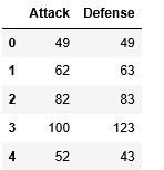
from sklearn.preprocessing import PolynomialFeatures

#构造二次交互项

pf = PolynomialFeatures(degree=2, interaction_only=False, include_bias=False)

res = pf.fit_transform(atk_def)

res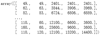
#加入到数据框中

intr_features = pd.DataFrame(res, columns=['Attack', 'Defense', 'Attack^2', 'Attack x Defense', 'Defense^2'])

intr_features.head(5) 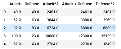
有同学可能会问,我怎么知道列的名称呢?可以这么看:
pd.DataFrame(pf.powers_, columns=['Attack_degree', 'Defense_degree'])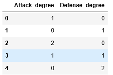
也就是说哪个是一次项哪些是二次项哪些是交互项都可以看出来。pf自从用了fit_transform之后,就记录了这份数据构造二次项的模式,后面要从新使用就可以用transform函数了。
new_df = pd.DataFrame([[95, 75],[121, 120], [77, 60]],

                      columns=['Attack', 'Defense'])

new_df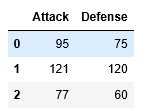
new_res = pf.transform(new_df)

new_intr_features = pd.DataFrame(new_res,

                                 columns=['Attack', 'Defense',

                                          'Attack^2', 'Attack x Defense', 'Defense^2'])

new_intr_features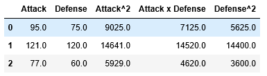
分箱
本质上是根据数值,把观测进行等级分类,比如60分以下判定为不及格,90分以上为优秀,就是简单的分箱。
#读数据

fcc_survey_df = pd.read_csv(file_path + 'datasets/fcc_2016_coder_survey_subset.csv', encoding='utf-8')

fcc_survey_df[['ID.x', 'EmploymentField', 'Age', 'Income']].head()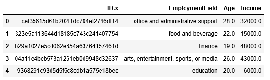
fig, ax = plt.subplots()

fcc_survey_df['Age'].hist(color='#A9C5D3')

ax.set_title('Developer Age Histogram', fontsize=12)

ax.set_xlabel('Age', fontsize=12)

ax.set_ylabel('Frequency', fontsize=12)
Text(0, 0.5, 'Frequency')
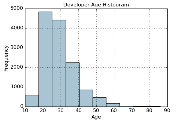
根据上面的分布图,进行分箱,也就是说10到20岁统一标为1。
fcc_survey_df['Age_bin_round'] = np.array(np.floor(np.array(fcc_survey_df['Age']) / 10.))

fcc_survey_df[['ID.x', 'Age', 'Age_bin_round']].iloc[1071:1076]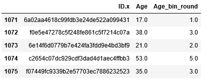
或者我们可以自定义自己的分箱范围标准:

bin_ranges = [0, 15, 30, 45, 60, 75, 100]

bin_names = [1, 2, 3, 4, 5, 6]

#首先看每个记录落在哪一个我们定义好的范围

fcc_survey_df['Age_bin_custom_range'] = pd.cut(np.array(fcc_survey_df['Age']),

                                               bins=bin_ranges)

#给我们定义好的范围进行数值编号

fcc_survey_df['Age_bin_custom_label'] = pd.cut(np.array(fcc_survey_df['Age']),

                                               bins=bin_ranges, labels=bin_names)

#观察我们整理好的数据框

fcc_survey_df[['ID.x', 'Age', 'Age_bin_round',

               'Age_bin_custom_range', 'Age_bin_custom_label']].iloc[1071:1076]
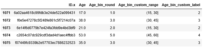
上面的意思是,0-15属于1级,30-45则属于3级,以此类推。
另一种分箱标准,就是采用分位数,比如四分位数。我们先看看数据,我们会对收入变量进行分箱。
fcc_survey_df[['ID.x', 'Age', 'Income']].iloc[4:9]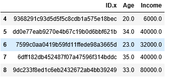
fig, ax = plt.subplots()
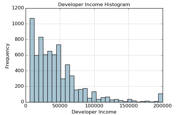
fcc_survey_df['Income'].hist(bins=30, color='#A9C5D3')
ax.set_title('Developer Income Histogram', fontsize=12)
ax.set_xlabel('Developer Income', fontsize=12)
ax.set_ylabel('Frequency', fontsize=12)Text(0, 0.5, 'Frequency')
#计算收入的分位数分别是多少

quantile_list = [0, .25, .5, .75, 1.]

quantiles = fcc_survey_df['Income'].quantile(quantile_list)

quantiles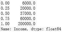
#在图中标出分位数的位置

fig, ax = plt.subplots()

fcc_survey_df['Income'].hist(bins=30, color='#A9C5D3')

for quantile in quantiles:

    qvl = plt.axvline(quantile, color='r')

ax.legend([qvl], ['Quantiles'], fontsize=10)

ax.set_title('Developer Income Histogram with Quantiles', fontsize=12)

ax.set_xlabel('Developer Income', fontsize=12)

ax.set_ylabel('Frequency', fontsize=12)
Text(0, 0.5, 'Frequency')

#根据分位数进行分箱特征提取

quantile_labels = ['0-25Q', '25-50Q', '50-75Q', '75-100Q']

fcc_survey_df['Income_quantile_range'] = pd.qcut(fcc_survey_df['Income'],

                                                 q=quantile_list)

fcc_survey_df['Income_quantile_label'] = pd.qcut(fcc_survey_df['Income'],

                                                 q=quantile_list, labels=quantile_labels)

fcc_survey_df[['ID.x', 'Age', 'Income',

               'Income_quantile_range', 'Income_quantile_label']].iloc[4:9]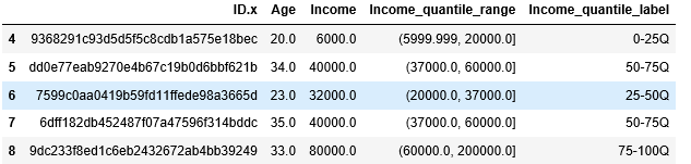
数学变换
我们这里提到的数学变化,基本都是因为数据不服从正态性,通过变化让数据服从正态分布,这样我们才能够用一些模型进行拟合。比如线性回归就需要数据服从正态性分布,如果有偏的话结果就会不可信。这里我们介绍对数变换和Box-Cox变换。
对数变换
我们可以看到,上面一个例子中收入是不服从左右对称的正态分布的,我们用对数变换看看是否起到效果。
fcc_survey_df['Income_log'] = np.log((1+ fcc_survey_df['Income']))   #为什么加1?如果有人收入为0那么就会出问题了。

fcc_survey_df[['ID.x', 'Age', 'Income', 'Income_log']].iloc[4:9]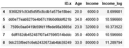
income_log_mean = np.round(np.mean(fcc_survey_df['Income_log']), 2)

fig, ax = plt.subplots()

fcc_survey_df['Income_log'].hist(bins=30, color='#A9C5D3')

plt.axvline(income_log_mean, color='r')

ax.set_title('Developer Income Histogram after Log Transform', fontsize=12)

ax.set_xlabel('Developer Income (log scale)', fontsize=12)

ax.set_ylabel('Frequency', fontsize=12)

ax.text(11.5, 450, r'$\mu$='+str(income_log_mean), fontsize=10)
Text(11.5, 450, '$\\mu$=10.43')

Box-Cox变换
做这个变换之前,首先要确定一个lambda值,不过建议傻瓜式复制就好,我们的任务只是要得到能够服从正态分布的一列变量而已。
income = np.array(fcc_survey_df['Income'])

income_clean = income[~np.isnan(income)]

l, opt_lambda = spstats.boxcox(income_clean)

print('Optimal lambda value:', opt_lambda)
Optimal lambda value: 0.11799123945557663
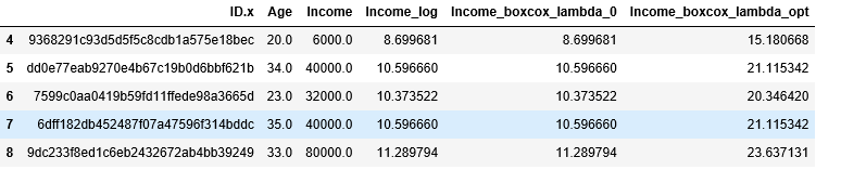
fcc_survey_df['Income_boxcox_lambda_0'] = spstats.boxcox((1+fcc_survey_df['Income']),

                                                         lmbda=0)

fcc_survey_df['Income_boxcox_lambda_opt'] = spstats.boxcox(fcc_survey_df['Income'],

                                                           lmbda=opt_lambda)

fcc_survey_df[['ID.x', 'Age', 'Income', 'Income_log',

               'Income_boxcox_lambda_0', 'Income_boxcox_lambda_opt']].iloc[4:9]
income_boxcox_mean = np.round(np.mean(fcc_survey_df['Income_boxcox_lambda_opt']), 2)

fig, ax = plt.subplots()

fcc_survey_df['Income_boxcox_lambda_opt'].hist(bins=30, color='#A9C5D3')

plt.axvline(income_boxcox_mean, color='r')

ax.set_title('Developer Income Histogram after Box–Cox Transform', fontsize=12)

ax.set_xlabel('Developer Income (Box–Cox transform)', fontsize=12)

ax.set_ylabel('Frequency', fontsize=12)

ax.text(24, 450, r'$\mu$='+str(income_boxcox_mean), fontsize=10)
Text(24, 450, '$\\mu$=20.65')

这里计算了lambda为0,以及为最优值的Box-Cox转换值。