本篇是集成方法系列(1)---bagging方法。
首先简单介绍下scikit-learn,这是一个用python实现的机器学习库。它的特点如下:
简单高效,可以用于数据挖掘和数据分析;
人人可用,可以用于多种场景;
基于Numpy, SciPy 和matplotlib, 其中numpy和scipy是python实现的科学计算库,matplotlib是画图库;
开源,可商用----BSD lisense
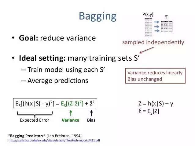
集成方法的目标是通过组合多个基准预测,然后利用学习算法使得集成算法相对单个预测具有更好的泛化能力或鲁棒性。
集成方法主要有两大家族:
平均法,即独立训练多个预测,然后对多个预测取平均得到最终预测。一般来讲,组合预测器通常比单个预测器要好,因为组合多个预测器会使得方差降低。
这类主要包含 bagging 方法,随机森林等。
boosting方法,需要建立一系列预测器,并且逐步缩小组合预测器的偏差。通过组合多个弱模型来得到一个强集成器。
这类方法主要包括Adaboost, GBDT等。
Bagging
集成算法中,bagging方法会构建一类算法,这些算法会在原始训练集中的随机自己中构建黑箱预测器,然后将这些预测器聚合起来,进而得到最终的预测器。这类方法在构建过程中借助于随机子集,然后将多个基准预测集成起来,如此一来可以减小基准预测器(比如决策树)的方差。很多情况下,bagging 方法是一种比较简单的并且可以提高单个模型性能的方式。bagging 方法可以预防过拟合,它在健壮和复杂模型中效果更好,而boosting方法则通常适用于弱模型。
Bagging 方法基于从原始训练集中随机选取子集,它会由于训练集中的随机子集采样方法不同而形式各异。一般可以分为以下四种:
如果随机子集是从训练集中随机采样而来的子集,则这种算法就是Pasting算法 [B1999]。
如果采样过程是有放回的,则这种方法就是Bagging方法 [B1996]。
如果采样过程是对特征集的随机采样,则这种方法称为随机子空间法 [H1998]。
如果采样既包含了样本随机,又包含了随机选择特征子集,则这种方法称为随机补丁法 [LG2012]。
在scikit-learn中,bagging 对应一个BaggingClassifier 或 BaggingRegressor,需要用户给定一个基准预测器和一个用来指定子集采样方法的参数。参数max_samples用来控制子集的大小,max_features用来控制特征子集中特征的个数,bootstrap 用来控制样本采样是否有放回,bootstrap_features用来控制特征采样是否有放回,泛化误差可以通过设置oob_score=True并且利用out-of-bag的样本来估计。
下面是一个如何初始化bagging集成算法的示例,其中基准预测器是KNeighborsClassifier,每个预测器利用50%的随机样本和50%的特征。
>>> from sklearn.ensemble import BaggingClassifier

>>> from sklearn.neighbors import KNeighborsClassifier

>>> bagging = BaggingClassifier(KNeighborsClassifier(),...                             max_samples=0.5, max_features=0.5)
完整示例如下:
print(__doc__)

# Author: Gilles Louppe <g.louppe@gmail.com>

# License: BSD 3 clause

import numpy as np    ##导入numpy python 中科学计算的库,类似matlab

import matplotlib.pyplot as plt    ## 画图库

from sklearn.ensemble import BaggingRegressor

from sklearn.tree import DecisionTreeRegressor

# Settings

n_repeat = 50       # Number of iterations for computing expectations

n_train = 50        # Size of the training set

n_test = 1000       # Size of the test set

noise = 0.1         # Standard deviation of the noise

np.random.seed(0)

# Change this for exploring the bias-variance decomposition of other

# estimators. This should work well for estimators with high variance (e.g.,

# decision trees or KNN), but poorly for estimators with low variance (e.g.,

# linear models).

estimators = [("Tree", DecisionTreeRegressor()),

             ("Bagging(Tree)", BaggingRegressor(DecisionTreeRegressor()))]

n_estimators = len(estimators)

# Generate data   生成数据

def f(x):

    x = x.ravel()


    return np.exp(-x ** 2) + 1.5 * np.exp(-(x - 2) ** 2)

def generate(n_samples, noise, n_repeat=1):

    X = np.random.rand(n_samples) * 10 - 5

    X = np.sort(X)


    if n_repeat == 1:

        y = f(X) + np.random.normal(0.0, noise, n_samples)

    else:

        y = np.zeros((n_samples, n_repeat))


        for i in range(n_repeat):
            # y的第i列


            y[:, i] = f(X) + np.random.normal(0.0, noise, n_samples)


    X = X.reshape((n_samples, 1))


    return X, y

X_train = []

y_train = []

for i in range(n_repeat):

    X, y = generate(n_samples=n_train, noise=noise)

    X_train.append(X)

    y_train.append(y)

X_test, y_test = generate(n_samples=n_test, noise=noise,
                          n_repeat=n_repeat)

# Loop over estimators to compare

for n, (name, estimator) in enumerate(estimators):

    # Compute predictions

    y_predict = np.zeros((n_test, n_repeat))


    for i in range(n_repeat):

        estimator.fit(X_train[i], y_train[i])

        y_predict[:, i] = estimator.predict(X_test)


    # Bias^2 + Variance + Noise decomposition of the mean squared error

    y_error = np.zeros(n_test)


    for i in range(n_repeat):

        for j in range(n_repeat):

            y_error += (y_test[:, j] - y_predict[:, i]) ** 2


    y_error /= (n_repeat * n_repeat)


    y_noise = np.var(y_test, axis=1)

    y_bias = (f(X_test) - np.mean(y_predict, axis=1)) ** 2

    y_var = np.var(y_predict, axis=1)


    print("{0}: {1:.4f} (error) = {2:.4f} (bias^2) "

          " + {3:.4f} (var) + {4:.4f} (noise)".format(name,

                                                      np.mean(y_error),

                                                      np.mean(y_bias),

                                                      np.mean(y_var),

                                                      np.mean(y_noise)))


    # Plot figures   画图

    plt.subplot(2, n_estimators, n + 1)

    plt.plot(X_test, f(X_test), "b", label="$f(x)$")

    plt.plot(X_train[0], y_train[0], ".b", label="LS ~ $y = f(x)+noise$")


    for i in range(n_repeat):

        if i == 0:

            plt.plot(X_test, y_predict[:, i], "r", label="$\^y(x)$")

        else:

            plt.plot(X_test, y_predict[:, i], "r", alpha=0.05)


    plt.plot(X_test, np.mean(y_predict, axis=1), "c",

             label="$\mathbb{E}_{LS} \^y(x)$")


    plt.xlim([-5, 5])

    plt.title(name)


    if n == 0:

        plt.legend(loc="upper left", prop={"size": 11})


    plt.subplot(2, n_estimators, n_estimators + n + 1)

    plt.plot(X_test, y_error, "r", label="$error(x)$")

    plt.plot(X_test, y_bias, "b", label="$bias^2(x)$"),

    plt.plot(X_test, y_var, "g", label="$variance(x)$"),

    plt.plot(X_test, y_noise, "c", label="$noise(x)$")


    plt.xlim([-5, 5])

    plt.ylim([0, 0.1])


    if n == 0:

        plt.legend(loc="upper left", prop={"size": 11})

plt.show()
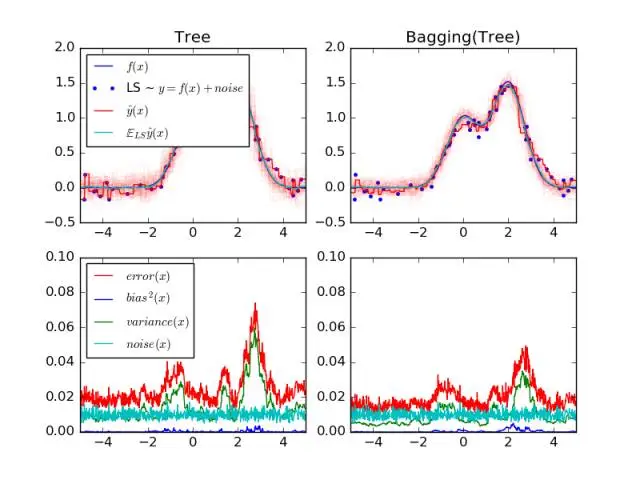
输出结果如下:
Tree: 0.0255 (error) = 0.0003 (bias^2)  + 0.0152 (var) + 0.0098 (noise)

Bagging(Tree): 0.0196 (error) = 0.0004 (bias^2)  + 0.0092 (var) + 0.0098 (noise)
输出图形如下:
参考资料
http://scikit-learn.org/stable/modules/ensemble.html#bagging-meta-estimator
http://scikit-learn.org/stable/auto_examples/ensemble/plot_bias_variance.html#example-ensemble-plot-bias-variance-py
[B1999]L. Breiman, “Pasting small votes for classification in large databases and on-line”, Machine Learning, 36(1), 85-103, 1999.
[B1996]L. Breiman, “Bagging predictors”, Machine Learning, 24(2), 123-140, 1996.
[H1998]T. Ho, “The random subspace method for constructing decision forests”, Pattern Analysis and Machine Intelligence, 20(8), 832-844, 1998.
[LG2012]G. Louppe and P. Geurts, “Ensembles on Random Patches”, Machine Learning and Knowledge Discovery in Databases, 346-361, 2012.
