机器学习实战之决策树（三）

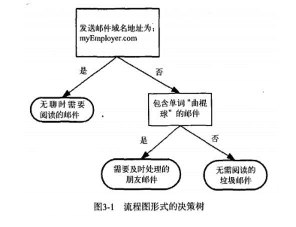
正方形代表判断模块(decision block) ，椭圆代表终止模块（terminating block），表示已经得到结论，可以终止运动。

决策树的优势在于数据形式容易理解。决策树的很多任务都是为了数据中所蕴含的知识信息。决策树可以使用不熟悉的数据集合，并从中提取出一系列规则，机器学习算法最终将使用这些机器从数据集中创造的规则。

3.1决策树的构造

优点：计算复杂度不高，输出结果易于理解，对中间值的缺失不敏感，可以处理不相关特征数据。

缺点：可能会产生过度匹配的问题。

适用数据类型：数值型和标称型。

1.先讨论数学上如何使用信息论划分数据集；

2.编写代码将理论应用到具体的数据集上；

3.编写代码构建决策树；

创建分支的伪代码函数createBranch() 

检测数据集中的每个子项是否属于同一分类：

    If so return 类标签 ：

    Else

        寻找划分数据集的最好特征

        划分数据集

        创建分支节点

            for 每个划分的子集

                调用函数createBranch 并增加返回结果到分支节点中

        return   分子节点

上面的伪代码createBranch是一个递归函数，在倒数第二行直接调用它子集、

决策树一般流程

1. 收集数据：可以直接使用任何方法
2. 准备数据：构造算法只适用于标称型数据，因此数值型数据必须离散化。
3. 分析数据：可以使用任何方法，构造完树以后，我们应该检查图形是否符合预期。
4. 训练算法：构造数的数据结构。
5. 测试算法：使用经验树计算错误概率
6. 使用算法：此步骤可以适应于任何监督学习算法，而使用决策树可以更好的理解数据的内在含义。

本次我们使用ID3算法来划分数据集。每次划分数据集的时我们只选取一个特征值。

决策树学习采用的是自顶向下的递归方法，其基本思想是以信息熵为度量构造一棵熵值下降最快的树，到叶子节点处的熵值为零，此时每个叶节点中的实例都属于同一类。

3.1.1 信息增益

划分数据集的大原则是 ：将无序的数据变得有序。

组织杂乱无章数据的一种方法就是使用信息论度量信息，信息论是量化处理信息的分支科学。

在划分数据集之前之后的信息发生的变化称之为信息增益，知道如何计算信息增益，我们就可以计算每个特征的值划分数据集获得的信息增益，获得信息增益最高的特征就是最好的选择。

集合信息的度量方式称之为 香农熵。

熵

熵是信息论中的概念，用来表示集合的无序程度，熵越大表示集合越混乱，反之则表示集合越有序。熵的计算公式为：

E = -P * log2P

熵定义为信息的期望值。那什么是信息呢？如果待分类的事务可能划分在多个分类之中，负荷xi的信息定义为：

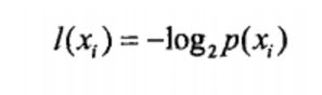
其中，p(xi)是选择分类的概率。

为了计算熵，我们需要计算所有类别的

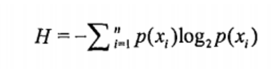
其中n是分类的数目。

接下来我们将使用pythoon计算信息熵，去度量数据集的无序程度，创建名为trees.py的文件。

from math import log



def calcShannonEnt(dataSet):

    #计算数据集中实例的总数

    numEntries = len(dataSet)

    #创建一个数据字典

    labelCounts = {}

    

    for featVec in dataSet:

        #取键值最后一列的数值的最后一个字符串

        currentLabel = featVec[-1]

        #键值不存在就使当前键加入字典

        if currentLabel not in labelCounts.keys():

            labelCounts[currentLabel] = 0

            labelCounts[currentLabel] += 1

    shannonEnt = 0.0

    for key in labelCounts:

        prob = float(labelCounts[key])/numEntries

        #以2为底求对数

        shannonEnt -= prob * log(prob,2)

    return shannonEnt

我们输入 一个数据来测试一下。

In [65]: import trees



In [67]: reload(trees)

Out[67]: <module 'trees' from 'trees.py'>



In [69]: def createDatSet():

    ...: dataSet = [[1,1,'yes'],

    ...: [1,1,'yes'],

    ...: [1,0,'no'],

    ...: [0,1,'no'],

    ...: [0,1,'no']]

    ...: labels = ['no surfacing','flippers']

    ...: return dataSet,labels

    ...:



In [70]: myDat,labels = trees.createDatSet()



In [71]: myDat

Out[71]: [[1, 1, 'yes'], [1, 1, 'yes'], [1, 0, 'no'], [0, 1, 'no'], [0, 1, 'no']]



In [72]: trees.calcShannonEnt(myDat)

Out[72]: 0.9709505944546686

熵越高，混合的数据就越多。

我们可以向数据集中添加更多的分类，以此来观测熵是如何变化的。

In [95]: myDat[0][-1]='maybe'



In [96]: myDat

Out[96]: [[1, 1, 'maybe'], [1, 1, 'yes'], [1, 0, 'no'], [0, 1, 'no'], [0, 1, 'no']]



In [97]: trees.calcShannonEnt(myDat)

Out[97]: 1.3709505944546687

3.1.2 划分数据集

分类算法除了要度量数据集的无序程度（信息熵），还需要划分数据集，度量划分数据集的熵。以便于判断当前是否正确划分了数据集。

我们队每个特征划分一次数据集的结果计算一次信息熵，然后去判断按照哪个特征划分数据集是最好的划分方式。

代码 ： 按照给定的特征划分数据集

#dataSet:待划分的数据集

#axis划分数据集的特征

#特征的返回值

def splitDataSet(dataSet,axis,value):

    #创建新的list对象

    retDataSet=[]

    for featVec in dataSet:

        if featVec[axis] == value:

            reducedFeatVec = featVec[:axis]

            reducedFeatVec.extend(featVec[axis+1：])

            retDataSet.append(reducedFeatVec)

    return retDataSet

上述代码append和extend方法，区别如下：

In [18]: a = [1,2,3]



In [19]: b = [4,5,6]



In [20]: a.append(b)



In [21]: a

Out[21]: [1, 2, 3, [4, 5, 6]]



In [22]: a = [1,2,3]



In [23]: b = [4,5,6]



In [24]: a.extend(b)



In [25]: a

Out[25]: [1, 2, 3, 4, 5, 6]

测试一下划分数据集的代码：

In [35]: reload(trees)

Out[35]: <module 'trees' from 'trees.py'>



In [36]: myDat,labels = trees.createDatSet()



In [37]: myDat

Out[37]: [[1, 1, 'yes'], [1, 1, 'yes'], [1, 0, 'no'], [0, 1, 'no'], [0, 1, 'no']]



In [38]: trees.splitDataSet(myDat,0,1)

Out[38]: [[1, 'yes'], [1, 'yes'], [0, 'no']]



In [39]: trees.splitDataSet(myDat,0,0)

Out[39]: [[1, 'no'], [1, 'no']]

记下来我们会遍历整个数据集，循环计算香农熵和splitDataSet()函数，找到最好的特征划分方式。熵计算会得出如何划分数据集是最好的数据组织方式。

def choooseBestFeatureToSplit(dataSet):

    numFeatures = len(dataSet[0]) -1

    baseEntropy = calcShannonEnt(dataSet)

    bestInfoGain = 0.0

    beatFeature =-1

    for i in range(numFeatures):

        #创建唯一的分类标签列表

        #取dataSet的第i个数据的第i个数据，并写入列表

        featList = [example[i] for example in dataSet]

        #将列表的数据集合在一起，并去重

        uniqueVals = set(featList)

        newEntropy = 0.0

        #计算每种划分方式的信息熵

        for value in uniqueVals:

            subDataSet = splitDataSet(dataSet,i,value)

            prob = len(subDataSet)/float(len(dataSet))

            newEntropy += prob * calcShannonEnt(subDataSet)

        infoGain = baseEntropy - newEntropy

        #计算好信息熵增益

        if (infoGain > bestInfoGain):

            bestInfoGain = infoGain

            bestFeature = i

    return bestFeature

上述代码实现选取特征，划分数据集，计算出最好的划分数据集的特征。

在函数的调用的数据中满足一定的要求：

（1） 数据必须是一种由列表元素组成的列表，且所有的列表元素具有相同的数据长度。

（2） 数据最后一列或每个实例的最后一个元素是当前实例的类别标签。

测试代码：

In [179]: reload(trees)



In [179]: Out[179]: <module 'trees' from 'trees.py'>



In [180]: trees.choooseBestFeatureToSplit(myDat)

Out[180]: 0



In [181]: myDat

Out[181]: [[1, 1, 'yes'], [1, 1, 'yes'], [1, 0, 'no'], [0, 1, 'no'], [0, 1, 'no']]

根据上述的结果，第0个特征就是最好的用于划分数据集的特征。

3.1.3 递归构建决策树

目前我们已经给出了从数据集构造决策树算法所需要的子功能模块，工作原理如下：

得到原始数据集，然后基于最好的属性值划分数据集，由于特征值可能多于两个，因此可能存在大于两个分支的数据集划分。第一次划分之后，数据将被乡下传递到树分支的下一个节点，在这个节点上，可以再次划分数据。因此我们可以使用递归的原理来处理数据。

递归结束的条件是：程序遍历完所有划分数据集的属性，或者每个分支下的所有的实例都具有相同的分类。如果所有实例具有相同的分类，则得到一个叶子节点或者终止块。

在代码最前面，输入

import operator

并输入以下代码

# 得出次数最多的分类名称

def majorityCnt(classList):

    classCount = {}

    for vote in classList:

        if vote not in classCount.keys():

            calssCount[vote] = 0

        classCount[vote] +=1

    sortedClassConnt = sorted(calssCount.iteritems(),key=operator.itemgetter(1),reverse=True)

    return sortedClassConnt[0][0]

函数使用分类名称的列表，然后创创建键值为classList中唯一值得数据字典，字典对象存储了classList中每个类标签出现的频率，利用operator操作键值排序字典，返回出现次数最多的分类名称。

下面给出创建树的代码：

def createTree(dataSet,labels):

    classList = [example[-1] for example in dataSet]

    #类别完全相同则停止继续划分

    if classList.count(classList[0]) ==len(classList):

        return classList[0]

    #遍历完所有的特征时返回出现次数最多的类别

    if len(dataSet[0]) == 1:

        return majorityCnt(classList)

    bestFeat = chooseBestFeatureToSplit(dataSet)

    bestFeatLabel = labels[bestFeat]

    myTree = {bestFeatLabel:{}}

    del(labels[bestFeat])

    #得到列表包含的所有属性

    featValues = [example[bestFeat] for example in dataSet]

    uniqueVals = set(featValues)

    for value in uniqueVals:

        subLabels = labels[:]

        myTree[bestFeatLabel][value] = createTree(splitDataSet\

                            (dataSet,bestFeat,value),subLabels)

    return myTree

执行以下命令，测试代码：

In [185]: reload(trees)

Out[185]: <module 'trees' from 'trees.py'>



In [186]: myDat,labels=trees.createDataSet()



In [187]: myTree=trees.createTree(myDat,labels)



In [188]: myTree

Out[188]: {'no surfacing': {0: 'no', 1: {'flippers': {0: 'no', 1: 'yes'}}}}

3.2 在python中使用matplotlib注解绘制树形图

由于字典的表示形式不好理解，所以我们使用matplotlib这个库来创建树形图。

给出的字典形式并不容易理解。决策树的优点就是直观易于理解。

于是我们自己绘制树形图。

3.2.1 Matplotlib 注解

由于字典的表示形式不好理解，所以我们使用matplotlib这个库来创建树形图。

Matplotlib 提供了一个工具annotations，它可以在数据图形上添加文本注解。注解同城用于解释数据的内容。

在计算机科学中，图是一种数据结构，用于表示数学上的概念。

接下来我们创建新的treePlotter.py文件

3-5 使用文本注解绘制树节点

#定义文本框和箭头格式

decisionNode = dict(boxstyle = "sawtooth", fc = "0.8")

leafNode =  dict(boxstyle = "round4", fc = "0.8")

arrow_args = dict(arrowstyle = "<-")



#绘制带箭头的注解,createPlot.ax1是一个全局变量

def plotNode(nodeTxt,centerPt,parentPt,nodeType):

    createPlot.ax1.annotate(nodeTxt,xy = parentPt,xycoords = "axes fraction",\

    xytext = centerPt,textcoords = "axes fraction",va = "center",\

    ha = "center",bbox = nodeType ,arrowprops = arrow_args)



#创建新图形并清空绘图区，在绘图区绘制决策节点和叶节点

def createPlot():

    fig = plt.figure(1,facecolor = 'white')

    fig.clf()

    #createPlot.ax1是全局变量

    createPlot.ax1 = plt.subplot(111,frameon = False)

    plotNode('decisionNodes',(0.5,0.1),(0.1,0.5),decisionNode)

    plotNode('leafNodes',(0.8,0.1),(0.3,0.8),leafNode)

    plt.show()

测试一下代码：

In [6]: import treePlotter



In [7]: reload(treePlotter)

Out[7]: <module 'treePlotter' from 'treePlotter.py'>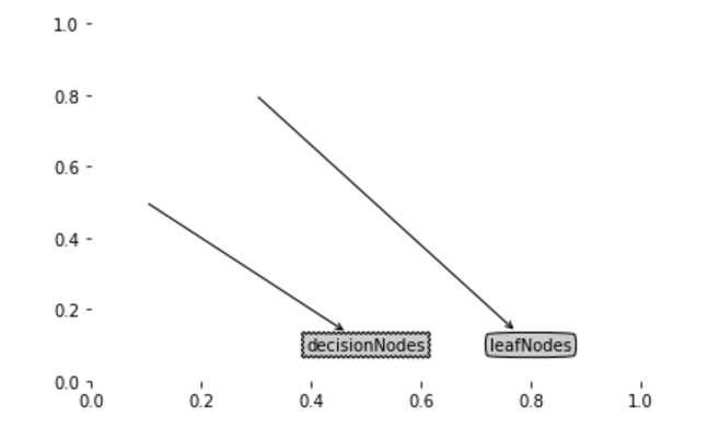

3.2.2 构造注解树

构造完整的一棵树，我们还需要知道，如何放置树节点，需要知道有多少个叶节点，便于确定x轴的长度，需要知道树多少层，便于正确确定y轴的高度。

获取叶节点的数目和树的层数

def getNumLeafs(myTree):

    numLeafs = 0

    firstStr = myTree.keys()[0]

    secondDict = myTree[firstStr]

    for key in secondDict.keys():

        #type()函数,测试节点的数据类型是否为字典

        if type(secondDict[key]).__name__ =='dict':

            numLeafs += getNumLeafs(secondDict[key])

        else:

            numLeafs += 1

    return numLeafs 



#计算遍历过程中的遇到判断节点的个数    

def getTreeDepth(myTree):

    maxDepth = 0

    firstStr = myTree.keys()[0]

    secondDict = myTree[firstStr]

    for key in secondDict.keys():

        if type(secondDict[key]).__name__ =='dict':

            thisDepth = 1 + getTreeDepth(secondDict[key])

        else:

            thisDepth = 1

        #如果达到子节点，则从递归调用中返回

        if thisDepth > maxDepth: 

            maxDepth = thisDepth

    return maxDepth

    



#我们为了便于测试，把这个树信息先存储进去

def retrieveTree(i):

    listOfTrees = [{'no surfacing': {0: 'no', 1: {'flippers': {0: 'no', 1: 'yes'}}}},

           {'no surfacing': {0: 'no', 1: {'flippers': {0: {'head':{0: 'no', 1: 'yes'}}, 1: 'no'}}}}]  

    return listOfTrees[i]

测试代码：

In [39]: import treePlotter



In [40]: reload(treePlotter)

Out[40]: <module 'treePlotter' from 'treePlotter.py'>



In [41]: myTree = treePlotter.retrieveTree(1)



In [42]: treePlotter.getTreeDepth(myTree)

Out[42]: 2



In [43]: treePlotter.getNumLeafs(myTree)

Out[43]: 3

我们继续将下面的代码添加到treePlotter.py中。

# plotTree函数



def plotMidText(cntrPt,parentPt,txtString):

    xMid = (parentPt[0] - cntrPt[0])/2.0 + cntrPt[0]

    yMid = (parentPt[1] - cntrPt[1])/2.0 + cntrPt[1]

    createPlot.ax1.text(xMid,yMid,txtString)



'''

全局变量plotTree.tatolW存储树的宽度

全局变量plotTree.tatolD存储树的高度

plotTree.xOff和plotTree.yOff追踪已经绘制的节点位置

'''   

def plotTree(myTree,parentPt,nodeTxt):

    #计算宽与高

    numLeafs = getNumLeafs(myTree)

    depth = getTreeDepth(myTree)

    firstStr = myTree.keys()[0]

    cntrPt = (plotTree.xOff+(1.0+float(numLeafs))/2.0/plotTree.totalW,plotTree.yOff)

    #标记子节点属性值

    plotMidText(cntrPt,parentPt,nodeTxt)

    plotNode(firstStr,cntrPt,parentPt,decisionNode)

    secondDict = myTree[firstStr]

    #减少y偏移

    plotTree.yOff = plotTree.yOff - 1.0/plotTree.totalD

    for key in secondDict.keys():

        if type(secondDict[key]).__name__ =='dict':

            plotTree(secondDict[key],cntrPt,str(key))

        else:

            plotTree.xOff = plotTree.xOff + 1.0/plotTree.totalW

            plotNode(secondDict[key],(plotTree.xOff,plotTree.yOff),cntrPt,leafNode)

            plotMidText((plotTree.xOff,plotTree.yOff),cntrPt,str(key))

    plotTree.yOff = plotTree.yOff + 1.0/plotTree.totalD

#这个是真正的绘制，上边是逻辑的绘制

def createPlot(inTree):

  fig = plt.figure(1, facecolor='white')

  fig.clf()

  axprops = dict(xticks=[], yticks=[])

  createPlot.ax1 = plt.subplot(111, frameon=False)	

  plotTree.totalW = float(getNumLeafs(inTree))

  plotTree.totalD = float(getTreeDepth(inTree))

  plotTree.xOff = -0.5/plotTree.totalW; plotTree.yOff = 1.0;

  plotTree(inTree, (0.5,1.0), '')

  plt.show()

继续测试代码：

In [5]: import treePlotter



In [6]: reload(treePlotter)

Out[6]: <module 'treePlotter' from 'treePlotter.pyc'>



In [7]: myTree = treePlotter.retrieveTree(0)

In [8]: treePlotter.createPlot(myTree)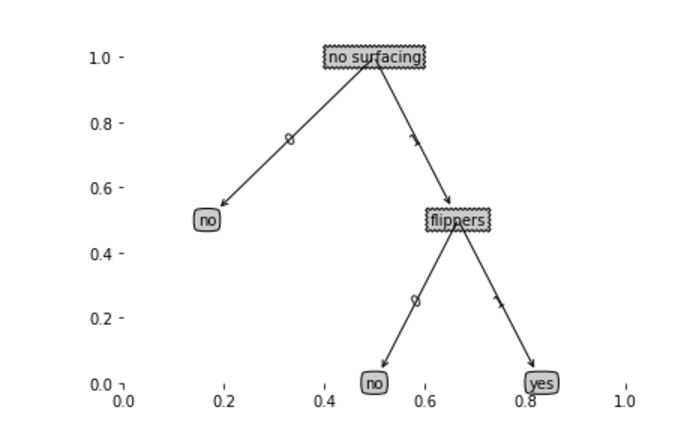

我们来变更一下字典来测试代码

In [10]: myTree['no surfacing'][3] = 'maybe'



In [11]: myTree

Out[11]: {'no surfacing': {0: 'no', 1: {'flippers': {0: 'no', 1: 'yes'}}, 3: 'maybe'}}



In [12]: treePlotter.createPlot(myTree)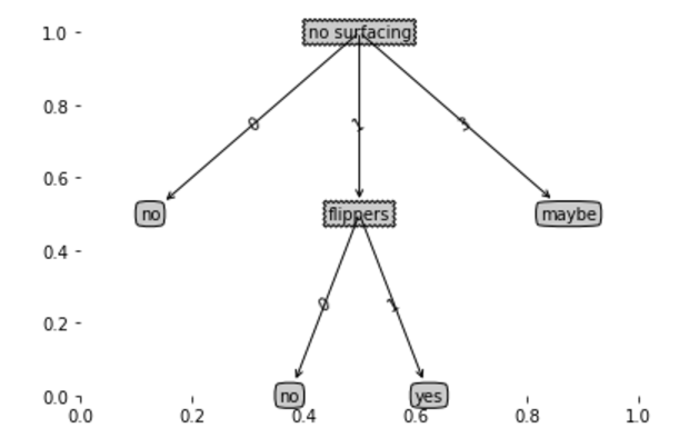

3.3 测试算法： 使用决策树执行分类

在trees.py中，添加下面的代码

#使用决策树的分类函数

def classify(inputTree,featLabels,testVec):

    firstStr = inputTree.keys()[0]

    secondDict = inputTree[firstStr]

    #将标签字符串转换为索引

    featIndex = featLabels.index(firstStr)

    for key in secondDict.keys():

        if testVec[featIndex] == key:

            if type(secondDict[key]).__name__ == 'dict':

                classLabel = classify(secondDict[key],featLabels,testVec)

            else:

                classLabel = secondDict[key]

    return classLabel  

我们来测试代码

In [11]: import trees



In [12]: reload(trees)

Out[12]: <module 'trees' from 'trees.pyc'>



In [14]: myDat,labels = trees.createDataSet()



In [15]: labels

Out[15]: ['no surfacing', 'flippers']



In [16]: myTree = treePlotter.retrieveTree(0)



In [17]: myTree

Out[17]: {'no surfacing': {0: 'no', 1: {'flippers': {0: 'no', 1: 'yes'}}}}



In [18]: trees.classify(myTree,labels,[1,1])

Out[18]: 'yes'



In [19]: trees.classify(myTree,labels,[1,0])

Out[19]: 'no'

将此结果与之前的图做比较，不难发现，结果相符。

3.3.2 使用算法 ：决策树的存储

构造决策树是一个很耗时的事情，如果数据集很大，将会非常耗时间。为此，我们调用python模块的pickle序列化对象。序列化对象可以在磁盘上保存文件，并在需要的时候读取出来。

#使用pickle模块存储决策树

def storeTree(inputTree,filename)        :

    import pickle

    fw = open(filename, 'w')

    pickle.dump(inputTree,fw)

    fw.close

    

def grabTree(filename):

    import pickle

    fr = open(filename)

    return pickle.load(fr)

测试代码：

In [22]: reload(trees)

Out[22]: <module 'trees' from 'trees.py'>



In [23]: trees.storeTree(myTree,r'E:\ML\ML_source_code\mlia\Ch03\classifierStorage.txt')



In [24]: trees.grabTree(r'E:\ML\ML_source_code\mlia\Ch03\classifierStorage.txt')

Out[24]: {'no surfacing': {0: 'no', 1: {'flippers': {0: 'no', 1: 'yes'}}}}

通过上面的代码，我们可以对数据分类时重新学习一遍。

3.4 示例：使用决策树预测隐形眼镜类型

眼科医生是如何判断患者需要佩戴的镜片类型的。

由于前面已经写好了算法模块：

我们载入本地的数据集之后，可以直接测试代码：

In [5]: import trees



In [6]: reload(trees)

Out[6]: <module 'trees' from 'trees.pyc'>



In [8]: import treePlotters



In [9]: reload(treePlotters)

Out[9]: <module 'treePlotters' from 'treePlotters.pyc'>



In [11]: fr = open(r'E:\ML\ML_source_code\mlia\Ch03\lenses.txt')



In [12]: lenses = [inst.strip().split('\t') for inst in fr.readlines()]



In [13]: lensesLabels = ['age','prescript','astigmatic','tearRate']



In [14]: lensesTree = trees.createTree(lenses,lensesLabels)



In [15]: lensesTree

Out[15]:

{'tearRate': {'normal': {'astigmatic': {'no': {'age': {'pre': 'soft',

'presbyopic': {'prescript': {'hyper': 'soft', 'myope': 'no lenses'}},

'young': 'soft'}},

'yes': {'prescript': {'hyper': {'age': {'pre': 'no lenses',

'presbyopic': 'no lenses',

'young': 'hard'}},

'myope': 'hard'}}}},

'reduced': 'no lenses'}}



In [17]: treePlotters.createPlot(lensesTree)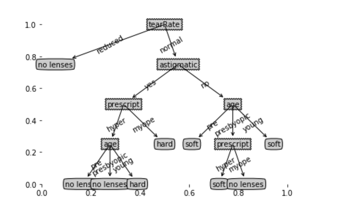

最终得到上面这个图，可是这些匹配选项可能太多了，我们将这些问题称之为过度匹配。

为了减少这个问题，我们可以裁剪决策树，去掉一些不必要的子节点。