Shiny包不同与R中其他包,它是由Rstudio公司打造用于让R用户便捷的构建web app,它兼容所有的HTML元素,Javascript,CSS,本文就shiny的一些简单知识进行说明。
1、基础知识
1.1 Panel
tabPanel 选项面板
mainPanel 主面板
sidebarPanel 侧边面板
titlePanel 标题面板(等价于 headerPanel)
coditionPanel 选项面板
inputPanel 输入面板(任意字符或HTML元素),等价于wellPanel
navlistPanel 导航面板
1.2 Widgets—app
每个wideget本身就是一个封装好的webapp函数
actionButton 动作按钮
checkboxGroupInput 复选框
checkboxInput 单选框
dateInput 日期输入
dataRangeInput 日期范围输入
fileInput 文件上传
helpText 帮助文档
numericInput 数字输入
radioButtons 一组 单选框
selectInput 待选盒
sliderInput 滑动条
submitButton 传送按钮
textInput 文本输入
1.3 act—app
htmlOutput HTML 代码
imageOutput 图像输出
plotOut put 图表输出
tableOutput 表格输出
textOutput 文本输出
uiOutput 原始HTML输出
verbatimTextout 逐字输出(相当于打印)
1.4 render—app
renderImage 图像
renderPlot 图表
renderPrint 打印
renderTable 数据框、矩阵、数组等其他表结构
renderText 字符
renderUI shiny的标签对象或是HTML
1.5 HTML
p 一段文字
h1 级别1的标题
h2 级别2的标题
h3 级别3的标题
h4 级别4的标题
h5 级别5的标题
h6 级别6的标题
a 一个超链接
div 具有某种风格的文本区域
br 一个换行符
span 具有某种统一风格的行内区域
pre 具有固定宽度的字体
code 一段格式化的代码块
img 一张图片
strong 粗体字
em 斜体字
HTML 直接以HTML代码样式通过的字符
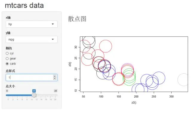
2、 一个简单例子
2.1 基本绘图风格
library(shiny)
# Define UI for application that draws a histogram
ui <- fluidPage(
headerPanel("mtcars data"),
#titlePanel("mtcars data"),
sidebarLayout(
sidebarPanel(
selectInput("var1", "x轴",
c("mpg" = "mpg",
"disp" = "disp",
"hp" = "hp"),
selected = 'mpg'),
selectInput("var2", "y轴",
c("mpg" = "mpg",
"disp" = "disp",
"hp" = "hp"),
selected = 'hp'
),
#submitButton("Update View"),
radioButtons('dist','颜色',
c('cyl'='cyl',
'gear'='gear',
'carb'='carb')),
numericInput("var3", "点样式", 0, min = 0, max = 25),
sliderInput("var4", "点大小",
min = 0, max = 20, value = 5
)
),
# Show a plot of the generated distribution
mainPanel(
h2('散点图'),
plotOutput("distPlot")
)
)
)
# Define server logic required to draw a histogram
server <- function(input, output) {
attach(mtcars)
z1 <- reactive({
switch(input$dist,
'cyl' = cyl,
'gear' =gear,
'carb' = carb)
})
z2 <- reactive({
switch(input$var1,
'mpg' = mpg,
'disp' = disp,
'hp' = hp)
})
z3 <- reactive({
switch(input$var2,
'mpg' = mpg,
'disp' = disp,
'hp' = hp)
})
output$distPlot <- renderPlot({
plot(z2(),z3(),
pch=input$var3,
cex=input$var4,
col=z1())
})
}
# Run the application
shinyApp(ui = ui, server = server)
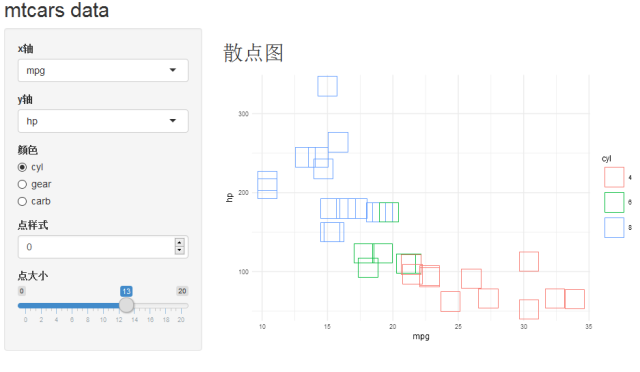
2.2 ggplot 绘制
library(shiny)
library(ggplot2)
# Define UI for application that draws a histogram
ui <- fluidPage(
titlePanel("mtcars data"),
sidebarLayout(
sidebarPanel(
selectInput("var1", "x轴",
c("mpg" = "mpg",
"disp" = "disp",
"hp" = "hp"),
selected = 'mpg'),
selectInput("var2", "y轴",
c("mpg" = "mpg",
"disp" = "disp",
"hp" = "hp"),
selected = 'hp'
),
#submitButton("Update View"),
radioButtons('dist','颜色',
c('cyl'='cyl',
'gear'='gear',
'carb'='carb')),
numericInput("var3", "点样式", 0, min = 0, max = 25),
sliderInput("var4", "点大小",
min = 0, max = 20, value = 5
)
),
# Show a plot of the generated distribution
mainPanel(
h2('散点图'),
plotOutput("distPlot")
)
)
)
# Define server logic required to draw a histogram
server <- function(input, output) {
output$distPlot <- renderPlot({
z1 <- switch(input$dist,
cyl = as.factor(mtcars$cyl),
gear = as.factor(mtcars$gear),
carb = as.factor(mtcars$carb))
z2 <- switch(input$var1,
mpg = mtcars$mpg,
disp = mtcars$disp,
hp = mtcars$hp)
z3 <- switch(input$var2,
mpg = mtcars$mpg,
disp = mtcars$disp,
hp = mtcars$hp)
ggplot(mtcars,aes(z2,z3,col=z1))+
geom_point(size=input$var4,
shape=input$var3)+
theme_minimal()+
xlab(input$var1)+
ylab(input$var2)+
labs(col=input$dist)
})
}
# Run the application
shinyApp(ui = ui, server = server)
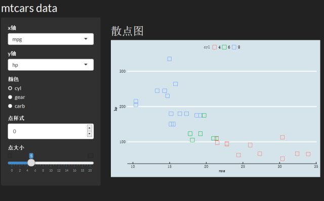
2.3 更换绘图主题为黑色(默认为Twitter风格)
library(shiny)
library(ggplot2)
library(shinythemes)
library(ggthemes)
# Define UI for application that draws a histogram
ui <- fluidPage(
theme=shinytheme("darkly"),
titlePanel("mtcars data"),
sidebarLayout(
sidebarPanel(
selectInput("var1", "x轴",
c("mpg" = "mpg",
"disp" = "disp",
"hp" = "hp"),
selected = 'mpg'),
selectInput("var2", "y轴",
c("mpg" = "mpg",
"disp" = "disp",
"hp" = "hp"),
selected = 'hp'
),
#submitButton("Update View"),
radioButtons('dist','颜色',
c('cyl'='cyl',
'gear'='gear',
'carb'='carb')),
numericInput("var3", "点样式", 0, min = 0, max = 25),
sliderInput("var4", "点大小",
min = 0, max = 20, value = 5
)
),
# Show a plot of the generated distribution
mainPanel(
h2('散点图'),
plotOutput("distPlot")
)
)
)
# Define server logic required to draw a histogram
server <- function(input, output) {
output$distPlot <- renderPlot({
z1 <- switch(input$dist,
cyl = as.factor(mtcars$cyl),
gear = as.factor(mtcars$gear),
carb = as.factor(mtcars$carb))
z2 <- switch(input$var1,
mpg = mtcars$mpg,
disp = mtcars$disp,
hp = mtcars$hp)
z3 <- switch(input$var2,
mpg = mtcars$mpg,
disp = mtcars$disp,
hp = mtcars$hp)
ggplot(mtcars,aes(z2,z3,col=z1))+
geom_point(size=input$var4,
shape=input$var3)+
theme_economist()+
xlab(input$var1)+
ylab(input$var2)+
labs(col=input$dist)
})
}
# Run the application
shinyApp(ui = ui, server = server)