使用Python进行线性回归

线性回归是最简单同时也是最常用的一个统计模型。线性回归具有结果易于理解，计算量小等优点。如果一个简单的线性回归就能取得非常不错的预测效果，那么就没有必要采用复杂精深的模型了。

今天，我们一起来学习使用Python实现线性回归的几种方法：

• 通过公式编写矩阵运算程序；
• 通过使用机器学习库sklearn;
• 通过使用statmodels库。

这里，先由简至繁，先使用sklearn实现，再讲解矩阵推导实现。

1.使用scikit-learn进行线性回归

设置工作路径

# 

import os

os.getcwd()

os.chdir('D:\my_python_workfile\Project\Writting')

加载扩展包

import pandas as pd

import numpy as np

import pylab as pl

import matplotlib.pyplot as plt

载入数据并可视化分析

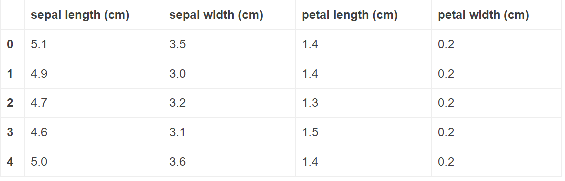
这里，为了简单起见，使用sklearn中自带的数据集鸢尾花数据iris进行分析，探索『花瓣宽』和『花瓣长』之间的线性关系。

from sklearn.datasets import load_iris

# load data

iris = load_iris()

# Define a DataFrame

df = pd.DataFrame(iris.data, columns = iris.feature_names)

# take a look

df.head()

#len(df)

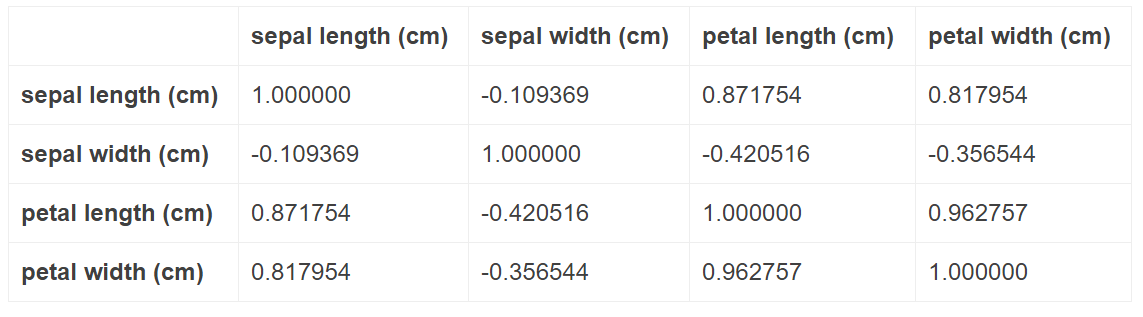
# correlation

df.corr()

# rename the column name 



df.columns = ['sepal_length','sepal_width','petal_length','petal_width']

df.columns

Index([u'sepal_length', u'sepal_width', u'petal_length', u'petal_width'], dtype='object')

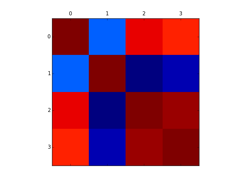
plt.matshow(df.corr())

由上面分析可知，花瓣长sepal length和花瓣宽septal width有着非常显著的相关性。

下面，通过线性回归进一步进行验证。

# save image

fig,ax = plt.subplots(nrows = 1, ncols = 1) 

ax.matshow(df.corr())

fig.savefig('./image/iris_corr.png')

建立线性回归模型

from sklearn.linear_model import LinearRegression

from sklearn.metrics import mean_squared_error



lr = LinearRegression()

X = df[['petal_length']]

y = df['petal_width']

lr.fit(X,y)

# print the result

lr.intercept_,lr.coef_

(-0.3665140452167297, array([ 0.41641913]))

# get y-hat

yhat = lr.predict(X = df[['petal_length']])



# MSE

mean_squared_error(df['petal_width'],yhat)

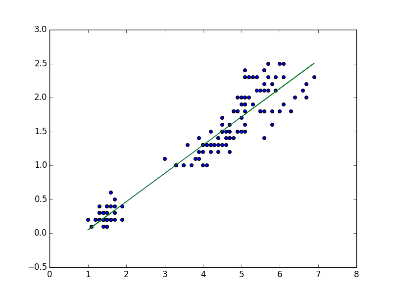
# lm plot

plt.scatter(df['petal_length'],df['petal_width'])

plt.plot(df['petal_length'],yhat)



#save image

plt.savefig('./image/iris_lm_fit.png')

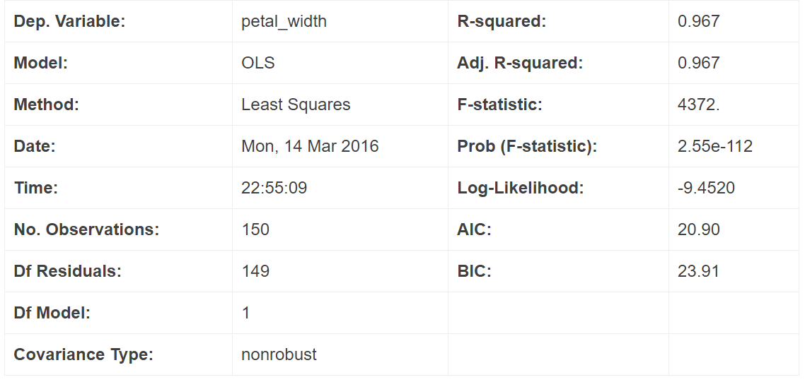
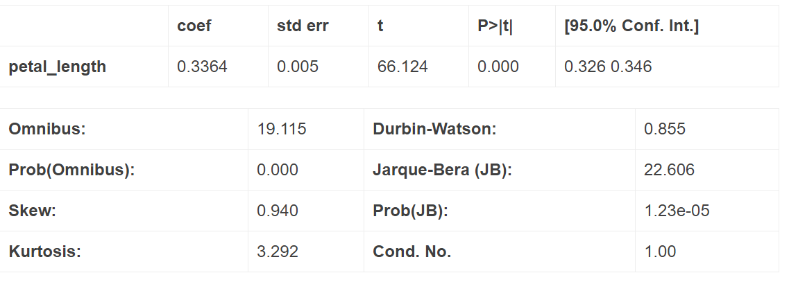
2.使用statmodels库

#import statsmodels.api as sm

import statsmodels.formula.api as sm



linear_model = sm.OLS(y,X)



results = linear_model.fit()



results.summary()

3.使用公式推导

线性回归，即是使得如下目标函数最小化：

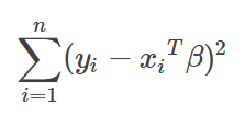
使用最小二乘法，不难得到ββ的估计：

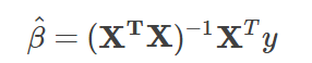
从而，我们可以根据此公式，编写求解β^β^的函数。

from numpy import *



#########################

# 定义相应的函数进行矩阵运算求解。

def standRegres(xArr, yArr):

    xMat = mat(xArr)

    yMat = mat(yArr).T

    xTx = xMat.T * xMat

    if linalg.det(xTx) == 0.0:

        print "this matrix is singular, cannot do inverse!"

        return NA

    else :

        ws = xTx.I * (xMat.T * yMat)

        return ws

# test

x0 = np.ones((150,1))

x0 = pd.DataFrame(x0)

X0 = pd.concat([x0,X],axis  = 1)

standRegres(X0,y)

matrix([[-0.36651405],

        [ 0.41641913]])

结果一致。

参考文献

• python中的线性回归

• Data Science in Python

• 『机器学习实战』