使用Python实现一个逻辑斯蒂回归

最近在整理代码，发现自己学习了好多代码都没发出来，有点空闲时间就弄一下；这个代码是我学习写算法的时候学习的，注释什么都已经加上了；

至于理论方面的话可以看看这个，没太多时间写了；这篇文章误差用的是似然估计，这个代码是使用是均方误差；这个是差异

https://ask.hellobi.com/blog/zhangjunhong0428/10359

# -*- coding: utf-8 -*-
import sys
reload(sys)
sys.setdefaultencoding('utf8')
import math
from numpy import *
import numpy
import time
import matplotlib.pyplot as plt
def load():
    train_x = []
    train_y = []
    file = open(r'E:\test/test.txt')
    for line in file.readlines():
       #将每行变成一个list
        line = line.strip().split()
         #参数1 是常量
        train_x.append([1.0, float(line[0]), float(line[1])])
        train_y.append(float(line[2]))
    return mat(train_x), mat(train_y).transpose()


#print test_x
#定义一个sigmoid函数,激活函数
def sigmoid(z):
    return 1.0/(1+numpy.exp(z))

# 使用一些可选的优化算法训练逻辑回归模型
# opts是一个字典，包括优化方式和最大迭代次数等。
def TrainLonRegeres(x,y,opts):
    startTime=time.time()
    #得到样本数和样本特征数
    NumSample,NumFeatures=shape(train_x)
    alpha = opts['alpha']
    maxIter = opts['maxIter']
    #构建三个特征的初始W值
    weights=ones((NumFeatures,1))
    #print train_x.transpose()
    ##开始应用梯度下降法求权重
    for k in range(maxIter):
       if opts["optimizeType"]=="gradDescent":#梯度下降法
           output=sigmoid(train_x*weights)
           #计算误差
           error=y-output
           #在计算梯度，并更新权重
           weights=weights- alpha*x.T*error
       elif opts['optimizeType'] == 'stocGradDescent':#随机梯度
           for i in range(NumSample):
               output=sigmoid(train_x[i, :] * weights)
               error=train_y[i]-output
               #print weights
               weights=weights-alpha*train_x[i,:].T*error
       elif opts['optimizeType'] == 'smoothStocGradDescent':  # 平滑后的随机梯度，根据前几次梯度进行一个平滑
           dataIndex = range(NumSample)
           #遍历整个样本
           for i in range(NumSample):
               #约束步长的变化
               alpha=4.0 / (1.0 + k + i) + 0.01
               #打乱数据的顺序
               randIndex = int(random.uniform(0, len(dataIndex)))
               output = sigmoid(train_x[randIndex, :] * weights)
               error=train_y[randIndex]-output
               #更新权重
               weights = weights - alpha * train_x[randIndex, :].transpose() * error
               #每次插入前删除优化后样本
               del (dataIndex[randIndex])
       else:
             raise NameError('Not support optimize method type!')
    print 'Congratulations, training complete! Took %fs!' % (time.time() - startTime)
    return weights
#测试训练的逻辑斯蒂回归结果如何
def testLogRegres(weights, test_x, test_y):
    NumSample,NumFeatures=shape(test_x)
    matchCount = 0
    for i in xrange(NumSample):
        predict= sigmoid(test_x[i, :] * weights)[0, 0]>0.5
        #判断是否为0或者1，如果是1则是TRUE
        if predict==bool(test_y[i,0]):
            matchCount += 1
        #计算准确率
    accuracy = float(matchCount) / NumSample
    print accuracy
    return accuracy


# 画图函数，通过这个来对比结果差异
def showLogRegres(weights, train_x, train_y):
    # 训练集必须都是矩阵类型
    numSamples, numFeatures = shape(train_x)
    if numFeatures != 3:
        print "Sorry! I can not draw because the dimension of your data is not 2!"
        return 1

        # draw all samples
    for i in xrange(numSamples):
        if int(train_y[i, 0]) == 0:
            plt.plot(train_x[i, 1], train_x[i, 2], 'or')
        elif int(train_y[i, 0]) == 1:
            plt.plot(train_x[i, 1], train_x[i, 2], 'ob')

            # draw the classify line
    min_x = min(train_x[:, 1])[0, 0]
    max_x = max(train_x[:, 1])[0, 0]
    weights = weights.getA()  # convert mat to array
    y_min_x = float(-weights[0] - weights[1] * min_x) / weights[2]
    y_max_x = float(-weights[0] - weights[1] * max_x) / weights[2]
    plt.plot([min_x, max_x], [y_min_x, y_max_x], '-g')
    plt.xlabel('X1');
    plt.ylabel('X2')
    plt.show()

train_x, train_y = load()
test_x = train_x
test_y = train_y
#定义一个学习步长和最大误差 gradDescent stocGradDescent smoothStocGradDescent
#maxIter 迭代次数
opts = {'alpha': 0.01, 'maxIter': 100, 'optimizeType': 'stocGradDescent'}
optimalWeights = TrainLonRegeres(train_x, train_y, opts)
## 测试集合
print "step 3: testing..."
accuracy = testLogRegres(optimalWeights, test_x, test_y)

## step 4: 展示结果
print "step 4: show the result..."
print 'The classify accuracy is: %.3f%%' % (accuracy * 100)
showLogRegres(optimalWeights, train_x, train_y)

结果得到如下：

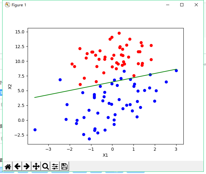
二分类上其实效果是可以的，附件有点坑人，不给上传txt格式的东西

数据集链接：https://pan.baidu.com/s/1fsM9H7xG9q9FRyV_V8IQbw