利用ComplexHeatmap绘制热图(一)

发表: 2018-08-22 浏览: 3463

数据分析 R语言

作者简介

taoyan：R语言中文社区特约作家，伪码农，R语言爱好者，爱开源。

简介

Complexheatmap是由顾祖光博士创建的绘制热图的R包，在他的GitHub有十分详细的小品文(Vignettes)说明。Complexheatmap是基于绘图系统grid，因此如果有相应grid的知识，学习起来应该更顺手！

设计

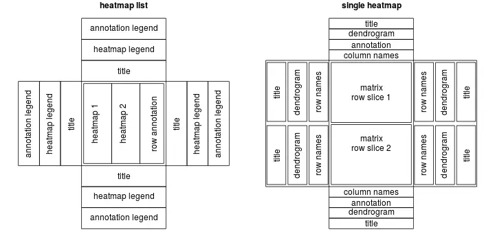
Complexheatmap提供了一套非常灵活的方法用于多热图也就是热图列表布局以及支持自定义注释绘图，一个热图列表包含若干热图以及注释信息

绘制单个热图

安装

包的安装就不细说了，有不懂的可以翻我以前的博客，里面有详细的教程，下面直接给出安装代码不解释

# installed from bioconductor

source("http://bioconductor.org/biocLite.R")

options(BioC_mirror="http://mirrors.ustc.edu.cn/bioc/")

biocLite("ComplexHeatmap")

# installed from GitHub

if(!require(devtools)){install.packages("devtools")}

devtools::install_github("jokergoo/ComplexHeatmap")

创建数据集

pacman::p_load(ComplexHeatmap, circlize)

set.seed(7)

mat <- cbind(rbind(matrix(rnorm(16, -1),4), matrix(rnorm(32, 1), 8)), rbind(matrix(rnorm(24, 1), 4), matrix(rnorm(48, -1), 8)))

mat <- mat[sample(nrow(mat), nrow(mat)), sample(ncol(mat), ncol(mat))]

rownames(mat) <- paste0("R", 1:12)

colnames(mat) <- paste0("C", 1:10)

绘图

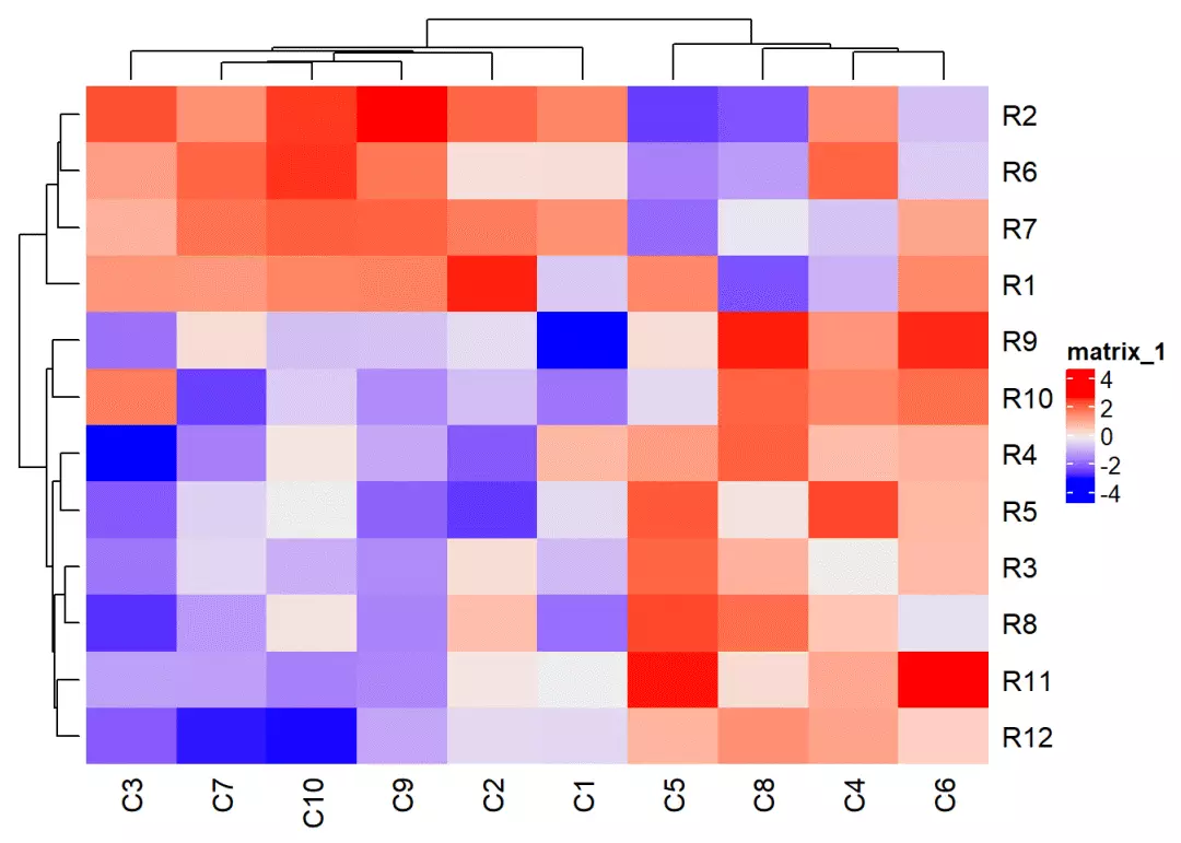
ComplexHeatmap绘制热图十分简单,使用默认参数

Heatmap(mat)

定制化

ComplexHeatmap十分灵活，可以自定义多种参数绘制热图

颜色

大多数情况下，绘制热图的矩阵都是连续性变量，通过提供颜色映射函数，我们可以自定义颜色，这主要是通过circlize包中的colorRamp2()函数来实现的,

mat2 <- matmat2[1,1] <- 100000Heatmap(mat2, col = colorRamp2(c(-3,0,3), c("green","white","red")), cluster_rows = FALSE, cluster_columns = FALSE)

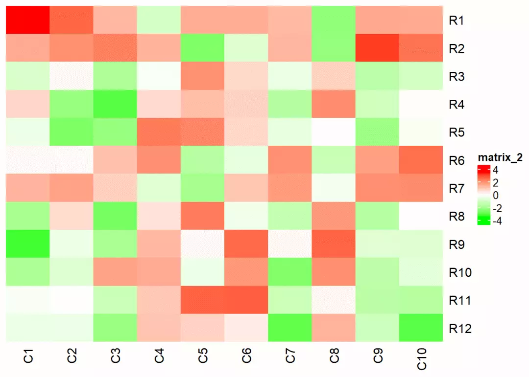
可以看出，ComplexHeatmap对于异常值也能显示出来，不会剔除掉

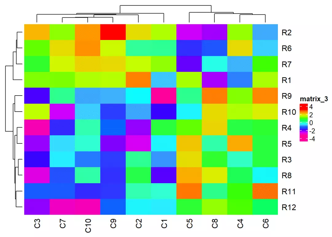
Heatmap(mat, col = rev(rainbow(10))

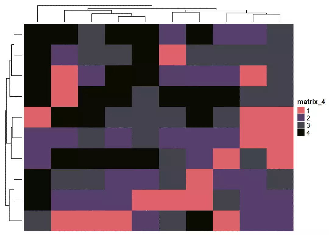
如果是离散型变量或者数值型、字符型变量的话，这时就需要特别指定颜色了

#离散型变量/数值型变量discrete_mat <- matrix(sample(1:4, 100, replace = TRUE), 10, 10)colors <- structure(circlize::rand_color(4), names=c("1","2","3","4"))Heatmap(discrete_mat, col = colors)

#字符型变量

character_mat <- matrix(sample(letters[1:4], 100, replace = TRUE), 10, 10)

colors <- structure(circlize::rand_color(4), names=letters[1:4])

Heatmap(character_mat, col = colors)

可以看出，对于离散型变量/数值型变量，默认对行/列进行聚类，而对于字符型变量，则不进行聚类

ComplexHeatmap允许数据中含有NA,只需要通过参数na_col来控制NA的颜色

mat_with_NA <- matmat_with_NA[sample(c(TRUE, FALSE), nrow(mat)*ncol(mat), replace = TRUE, prob = c(1,9))] <- NAHeatmap(mat_with_NA, na_col = "orange", clustering_distance_rows = "pearson")

ComplexHeatmap默认使用LAB颜色空间(LAB color space)，colorRamp2()提供了选择颜色空间的参数选项

f1 <- colorRamp2(seq(min(mat), max(mat), length=3), c("blue","#EEEEEE", "red"))f2 <- colorRamp2(seq(min(mat), max(mat), length=3), c("blue","#EEEEEE", "red"), space = "RGB")H1 <- Heatmap(mat, col = f1, column_title = "LAB color space")H2 <- Heatmap(mat, col = f2, column_title = "RGB color space")H1+H2

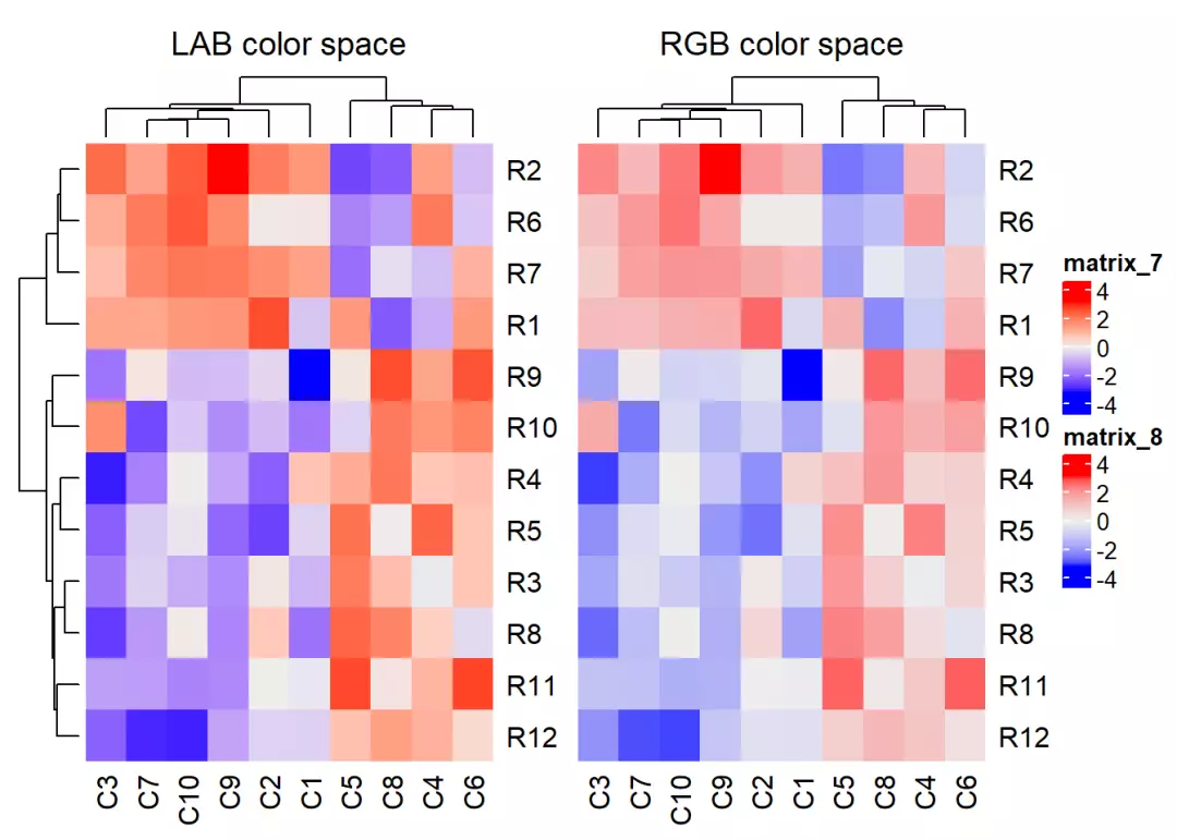
ComplexHeatmap提供了多种颜色空间选项，可以根据自身数据不断调整，选取合适的颜色空间

标题

一个热图的标题有：图标题、图例标题、行列标题等
Heatmap里提供的name参数默认的是图例的标题

Heatmap(mat, name = "legend")

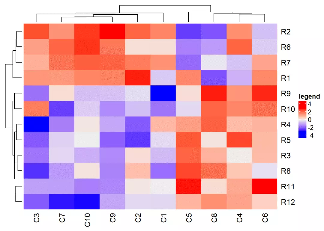
图里标题可以通过heatmap_legend_param()进行修改

Heatmap(mat, heatmap_legend_param = list(title="legend"))

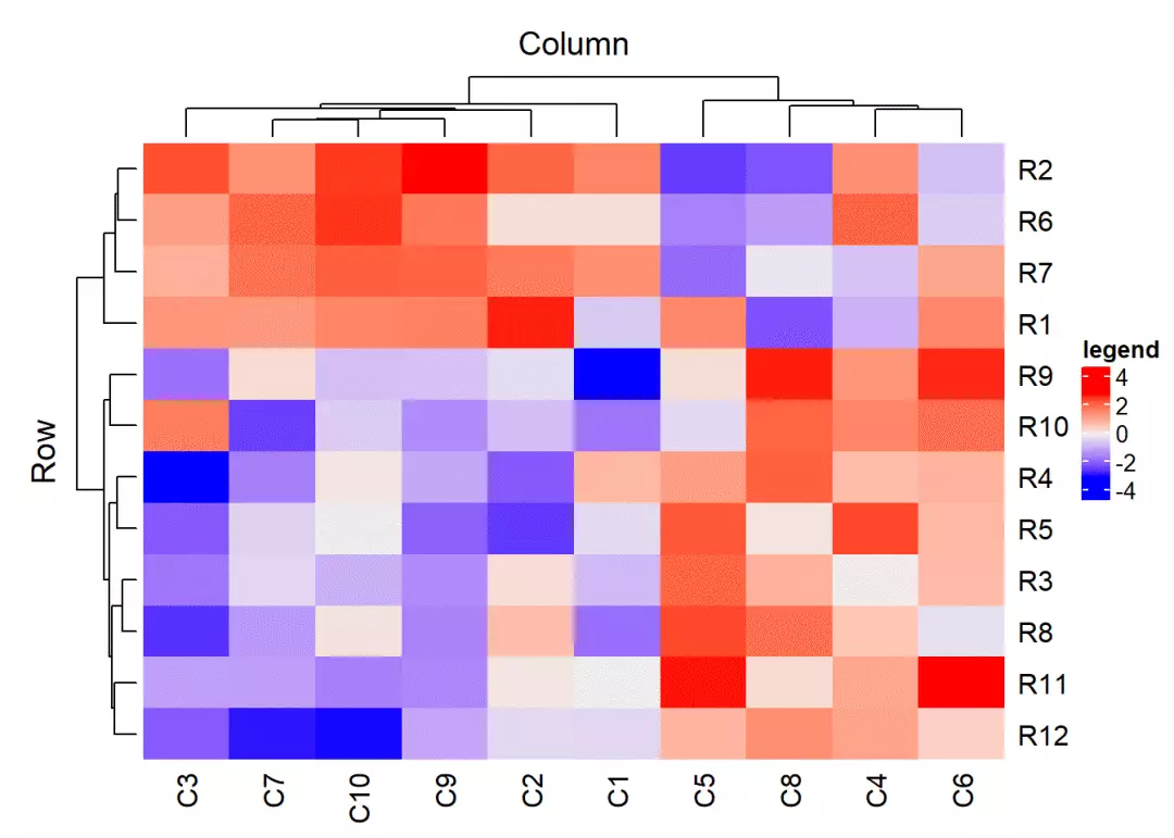
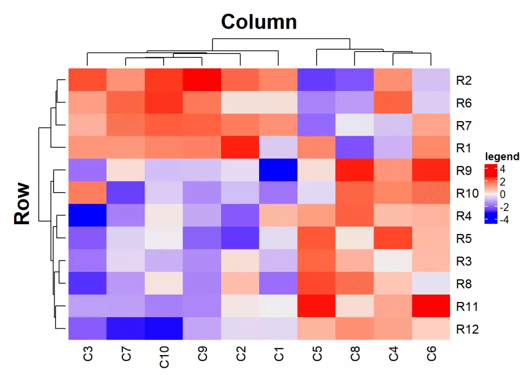
行列标题

Heatmap(mat, name = "legend", column_title = "Column", row_title = "Row")

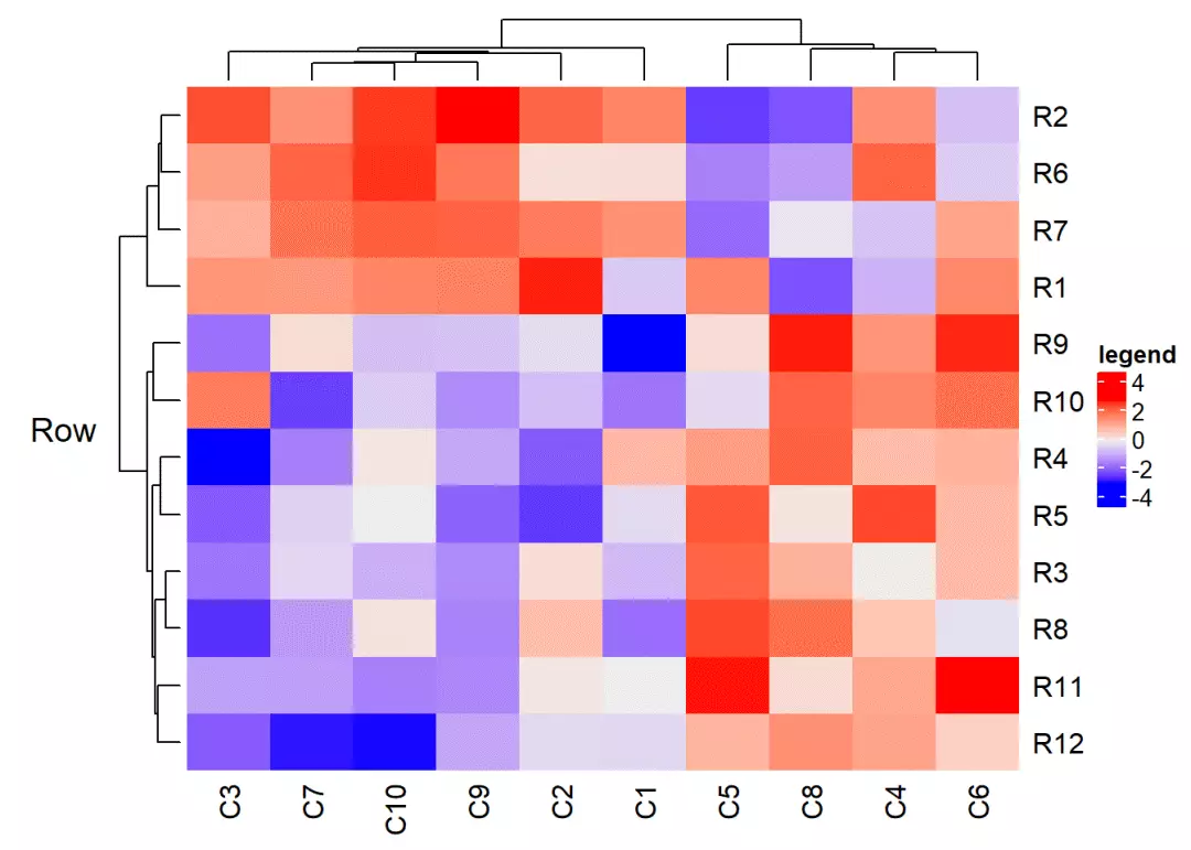
Heatmap(mat, name = "legend", column_title = "Column", column_title_side = "bottom")

如果需要修改图例参数，可以通过gpar()参数

Heatmap(mat, name = "legend",column_title = "Column", row_title = "Row", column_title_gp = gpar(fontsize=20, fontface="bold"), row_title_gp = gpar(fontsize=20, fontface="bold"))

标题可以旋转(水平或竖直)

SessionInfo

sessionInfo()

## R version 3.4.4 (2018-03-15)## Platform: x86_64-w64-mingw32/x64 (64-bit)## Running under: Windows 10 x64 (build 16299)## ## Matrix products: default## ## locale:## [1] LC_COLLATE=Chinese (Simplified)_China.936 ## [2] LC_CTYPE=Chinese (Simplified)_China.936 ## [3] LC_MONETARY=Chinese (Simplified)_China.936## [4] LC_NUMERIC=C ## [5] LC_TIME=Chinese (Simplified)_China.936 ## ## attached base packages:## [1] grid stats graphics grDevices utils datasets methods ## [8] base ## ## other attached packages:## [1] circlize_0.4.3 ComplexHeatmap_1.17.1## ## loaded via a namespace (and not attached):## [1] Rcpp_0.12.16 digest_0.6.15 rprojroot_1.3-2 ## [4] backports_1.1.2 pacman_0.4.6 magrittr_1.5 ## [7] evaluate_0.10.1 GlobalOptions_0.0.13 stringi_1.1.7 ## [10] GetoptLong_0.1.6 rmarkdown_1.9 RColorBrewer_1.1-2 ## [13] rjson_0.2.15 tools_3.4.4 stringr_1.3.0 ## [16] yaml_2.1.18 compiler_3.4.4 colorspace_1.3-2 ## [19] shape_1.4.4 htmltools_0.3.6 knitr_1.20