游戏用户流失预测数据分析

• 练习数据来源

谢佳标老师R语言游戏数据分析和挖掘中的第8章：用户流失预测数据.csv

• 数据分析方法

使用各种分类算法（二元logistic回归、决策树、随机森林、人工神经网络）

• 分析步骤

按照谢老师文章中的步骤，依次为：

1. 步骤1：数据转换：增加周活跃度和玩牌胜率等衍生指标。周活跃度＝登录总次数/7；玩牌胜率＝赢牌局数/玩牌局数;玩牌负率＝输牌局数/玩牌局数。
2. 步骤2：变量相关性分析：考虑因子变量的哑变量处理
3. 步骤3：10折交叉验证进行模型优化参数选择
   
4. 步骤4：构建决策树、随机森林、人工神经网络构建三种分类模型，并比较各分类器结果，选择最优分类器。

• 分析

##导入数据

说明：共1309条记录，13个字段。数据已经经过清洗，无缺失值，且变量属性无需修改。

> userchurn<-read.csv("E:\\R语言\\Game_DataMining_With_R-master\\data\\第8章\\用户流失预测数据.csv",header=T)

> str(userchurn)

'data.frame':	1309 obs. of  13 variables:

 $ 用户id    : int  1 2 3 4 5 6 7 8 9 10 ...

 $ 是否流失  : Factor w/ 2 levels "否","是": 2 1 1 2 2 2 1 2 2 1 ...

 $ 性别      : Factor w/ 2 levels "男","女": 1 1 1 1 1 1 1 1 1 1 ...

 $ 登录总次数: int  2 3 3 2 2 2 7 2 2 6 ...

 $ 站内好友数: int  1 5 1 0 1 0 1 0 0 0 ...

 $ 等级      : int  4 6 7 4 4 4 6 3 4 3 ...

 $ 积分      : int  0 5 8 0 0 0 26 0 0 20 ...

 $ 玩牌局数  : int  27 83 209 15 30 18 65 10 15 6 ...

 $ 赢牌局数  : int  4 40 56 4 3 8 10 3 8 2 ...

 $ 输牌局数  : int  0 43 153 0 0 0 55 0 7 4 ...

 $ 正常牌局  : int  0 11 0 16 30 18 64 10 15 6 ...

 $ 非正常牌局: int  0 0 0 0 0 0 1 0 0 0 ...

 $ 最高牌类型: int  0 7 8 0 0 0 7 0 8 4 ...

> summary(userchurn)

     用户id     是否流失  性别        登录总次数      站内好友数    

 Min.   :   1   否: 291   男:1057   Min.   : 2.00   Min.   : 0.000  

 1st Qu.: 328   是:1018   女: 252   1st Qu.: 2.00   1st Qu.: 0.000  

 Median : 655                       Median : 2.00   Median : 1.000  

 Mean   : 655                       Mean   : 2.81   Mean   : 1.341  

 3rd Qu.: 982                       3rd Qu.: 3.00   3rd Qu.: 2.000  

 Max.   :1309                       Max.   :11.00   Max.   :22.000  

      等级             积分            玩牌局数         赢牌局数      

 Min.   : 0.000   Min.   :  0.000   Min.   :   1.0   Min.   :   1.00  

 1st Qu.: 3.000   1st Qu.:  0.000   1st Qu.:   8.0   1st Qu.:   2.00  

 Median : 4.000   Median :  0.000   Median :  23.0   Median :   7.00  

 Mean   : 4.361   Mean   :  7.257   Mean   : 104.4   Mean   :  26.53  

 3rd Qu.: 5.000   3rd Qu.:  5.000   3rd Qu.:  63.0   3rd Qu.:  19.00  

 Max.   :16.000   Max.   :595.000   Max.   :7215.0   Max.   :2023.00  

    输牌局数          正常牌局         非正常牌局        最高牌类型    

 Min.   :   0.00   Min.   :    0.0   Min.   :  0.000   Min.   : 0.000  

 1st Qu.:   0.00   1st Qu.:    8.0   1st Qu.:  0.000   1st Qu.: 0.000  

 Median :   0.00   Median :   22.0   Median :  0.000   Median : 0.000  

 Mean   :  69.05   Mean   :  110.2   Mean   :  1.483   Mean   : 3.475  

 3rd Qu.:  29.00   3rd Qu.:   63.0   3rd Qu.:  0.000   3rd Qu.: 8.000  

 Max.   :6568.00   Max.   :12425.0   Max.   :284.000   Max.   :11.000  

##变量转换

> ##变量转换

> userchurn$周活跃度<-round(userchurn$登录总次数/7,3)

> userchurn$玩牌胜率<-round(userchurn$赢牌局数/userchurn$玩牌局数,3)

> userchurn$玩牌负率<-round(userchurn$输牌局数/userchurn$玩牌局数,3)

考虑到自己电脑对中文不太友好，后续建模时总是出现警告，所以尽量将汉字字符改为英文字符，字段名则不需要改。

> levels(userchurn$是否流失)<-c("0","1")##0表示不会，1表示会

> levels(userchurn$性别)<-c("M","F")

##相关性分析

> library(caret)

> userchurn_dummy<-dummyVars(~.,data=userchurn)

> userchurn_dummy_pre<-as.data.frame(predict(userchurn_dummy,userchurn))

> str(userchurn_dummy_pre)

'data.frame':	1309 obs. of  18 variables:

 $ 用户id    : num  1 2 3 4 5 6 7 8 9 10 ...

 $ 是否流失.0: num  0 1 1 0 0 0 1 0 0 1 ...

 $ 是否流失.1: num  1 0 0 1 1 1 0 1 1 0 ...

 $ 性别.M    : num  1 1 1 1 1 1 1 1 1 1 ...

 $ 性别.F    : num  0 0 0 0 0 0 0 0 0 0 ...

 $ 登录总次数: num  2 3 3 2 2 2 7 2 2 6 ...

 $ 站内好友数: num  1 5 1 0 1 0 1 0 0 0 ...

 $ 等级      : num  4 6 7 4 4 4 6 3 4 3 ...

 $ 积分      : num  0 5 8 0 0 0 26 0 0 20 ...

 $ 玩牌局数  : num  27 83 209 15 30 18 65 10 15 6 ...

 $ 赢牌局数  : num  4 40 56 4 3 8 10 3 8 2 ...

 $ 输牌局数  : num  0 43 153 0 0 0 55 0 7 4 ...

 $ 正常牌局  : num  0 11 0 16 30 18 64 10 15 6 ...

 $ 非正常牌局: num  0 0 0 0 0 0 1 0 0 0 ...

 $ 最高牌类型: num  0 7 8 0 0 0 7 0 8 4 ...

 $ 周活跃度  : num  0.286 0.429 0.429 0.286 0.286 0.286 1 0.286 0.286 0.857 ...

 $ 玩牌胜率  : num  0.148 0.482 0.268 0.267 0.1 0.444 0.154 0.3 0.533 0.333 ...

 $ 玩牌负率  : num  0 0.518 0.732 0 0 0 0.846 0 0.467 0.667 ...

##构建相关矩阵

说明：可以看出用户流失除了与性别不相关外，和其他变量都相关，其中和登录总数、周活跃度、最高牌类型、玩牌负率、等级相关性比较高

> cor<-cor(userchurn_dummy_pre[,2:3],userchurn_dummy_pre[,-c(1:3)])##本次分析主要是看是否流失字段与其他变量之间的相关性，所以需要筛选

> library(corrplot)

> corrplot(cor,method="ellipse")

##筛选变量

说明：由于周活跃度、玩牌胜率是通过其他字段转换而来，所以和涉及的字段存在着很强相关性。在后续的分析中，与谢老师分析的不一样的是，我直接剔除了登录总数、玩牌局数以及赢牌局数，输牌局数。

> user_select<-userchurn[,-c(1,4,8,9,10)]

##数据分区

训练集：测试集=7:3

> library(caret)

> ind<-createDataPartition(user_select$是否流失,times=1,p=0.7,list=F)

> train_data<-user_select[ind,]

> test_data<-user_select[-ind,]

##10折交叉验证选择模型优化参数

> control<-trainControl(method = "repeatedcv",number = 10,repeats = 3)

#c5.0模型参数选择

> library(C50)

> library(plyr)

> c5.0_train<-train(是否流失~.,data=train_data,method="C5.0",trControl=control)

说明：最优模型参数选择：trials = 1, model = rules and winnow= TRUE。

> c5.0_train

C5.0 



917 samples

 10 predictor

  2 classes: '0', '1' 



No pre-processing

Resampling: Cross-Validated (10 fold, repeated 3 times) 

Summary of sample sizes: 824, 826, 826, 825, 826, 824, ... 

Resampling results across tuning parameters:



  model  winnow  trials  Accuracy   Kappa    

  rules  FALSE    1      0.9197142  0.7703119

  rules  FALSE   10      0.9215339  0.7724119

  rules  FALSE   20      0.9193676  0.7667339

  rules   TRUE    1      0.9269606  0.7795767

  rules   TRUE   10      0.9164135  0.7518620

  rules   TRUE   20      0.9189300  0.7622875

  tree   FALSE    1      0.9255352  0.7854662

  tree   FALSE   10      0.9120892  0.7514866

  tree   FALSE   20      0.9145977  0.7562199

  tree    TRUE    1      0.9247787  0.7758407

  tree    TRUE   10      0.9185757  0.7670737

  tree    TRUE   20      0.9134872  0.7519007



Accuracy was used to select the optimal model using  the largest value.

The final values used for the model were trials = 1, model = rules and winnow

 = TRUE.

#randomForest模型参数选择

说明：最优模型参数选择：mtry = 6

> randomForest_train<-train(是否流失~.,data=train_data,method="rf",trControl=control)

> randomForest_train

Random Forest 



917 samples

 10 predictor

  2 classes: '0', '1' 



No pre-processing

Resampling: Cross-Validated (10 fold, repeated 3 times) 

Summary of sample sizes: 826, 824, 825, 826, 825, 824, ... 

Resampling results across tuning parameters:



  mtry  Accuracy   Kappa    

   2    0.9127843  0.7476679

   6    0.9200548  0.7704936

  10    0.9189798  0.7688598



Accuracy was used to select the optimal model using  the largest value.

The final value used for the model was mtry = 6.

#nnet模型参数选择

说明：最优模型参数选择：size = 1 and decay = 0.1

> nnet_train<-train(是否流失~.,data=train_data,method="nnet",trControl=control)

> nnet_train

Neural Network 



917 samples

 10 predictor

  2 classes: '0', '1' 



No pre-processing

Resampling: Cross-Validated (10 fold, repeated 3 times) 

Summary of sample sizes: 825, 825, 826, 826, 826, 824, ... 

Resampling results across tuning parameters:



  size  decay  Accuracy   Kappa    

  1     0e+00  0.8698903  0.5516198

  1     1e-04  0.8653639  0.4981789

  1     1e-01  0.9153212  0.7446841

  3     0e+00  0.9029149  0.7366187

  3     1e-04  0.9010198  0.7164779

  3     1e-01  0.9124069  0.7422376

  5     0e+00  0.9029703  0.7178035

  5     1e-04  0.9044032  0.7303573

  5     1e-01  0.9098426  0.7375306



Accuracy was used to select the optimal model using  the largest value.

The final values used for the model were size = 1 and decay = 0.1.

##模型构建

#构建c5.0决策树模型

> fit_c5.0<-C5.0(是否流失~.,data=train_data,trails=1,rules=T,control=C5.0Control(winnow = TRUE))

> summary(fit_c5.0)



Call:

C5.0.formula(formula = 是否流失 ~ ., data = train_data, trails = 1, rules =

 T, control = C5.0Control(winnow = TRUE))



C5.0 [Release 2.07 GPL Edition]  	Thu Aug 03 20:39:16 2017

-------------------------------

Class specified by attribute `outcome'

Read 917 cases (11 attributes) from undefined.data



3 attributes winnowed

Estimated importance of remaining attributes:

    176%  周活跃度

     16%  站内好友数

     11%  积分

      8%  正常牌局

     <1%  性别

     <1%  非正常牌局

     <1%  最高牌类型



Rules:

Rule 1: (5, lift 3.9)

	站内好友数 > 0

	站内好友数 <= 2

	积分 <= 6

	正常牌局 <= 8

	周活跃度 > 0.286

	->  class 0  [0.857]



Rule 2: (292/88, lift 3.1)

	周活跃度 > 0.286

	->  class 0  [0.697]



Rule 3: (625, lift 1.3)

	周活跃度 <= 0.286

	->  class 1  [0.998]



Rule 4: (621/26, lift 1.2)

	站内好友数 <= 2

	积分 <= 5

	->  class 1  [0.957]



Default class: 1

Evaluation on training data (917 cases):



	        Rules     

	  ----------------

	    No      Errors



	     4   60( 6.5%)   <<



	   (a)   (b)    <-classified as

	  ----  ----

	   183    21    (a): class 0

	    39   674    (b): class 1



	Attribute usage:

	100.00%	周活跃度

	 67.72%	站内好友数

	 67.72%	积分

	  0.55%	正常牌局

> ##训练集预测

> pre_c5.0_train<-predict(fit_c5.0,train_data,type="class")

> ##测试集预测

> pre_c5.0_test<-predict(fit_c5.0,test_data,type="class")

说明：混淆矩阵给出了交叉表的各种指标值。后续每个模型都会用到这一函数。可以在模型比较中，一次性对各模型混淆矩阵结果进行比较。

>t_c5.0_test<-confusionMatrix(pre_c5.0_test,test_data$是否流失)

> t_c5.0

Confusion Matrix and Statistics



          Reference

Prediction   0   1

         0  74  17

         1  13 288                                          

               Accuracy : 0.9235          

                 95% CI : (0.8925, 0.9478)

    No Information Rate : 0.7781          

    P-Value [Acc > NIR] : 9.13e-15                                                  

                  Kappa : 0.782           

 Mcnemar's Test P-Value : 0.5839                                                    

            Sensitivity : 0.8506          

            Specificity : 0.9443          

         Pos Pred Value : 0.8132          

         Neg Pred Value : 0.9568          

             Prevalence : 0.2219          

         Detection Rate : 0.1888          

   Detection Prevalence : 0.2321          

      Balanced Accuracy : 0.8974          

                                          

       'Positive' Class : 0     

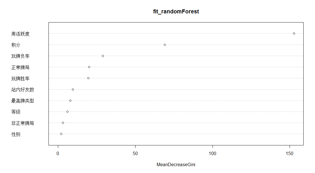
#构建随机森林

说明：对于模型构建最重要的变量依次为：周活跃率、积分、玩牌负率、正常牌局、玩牌胜率

> library(randomForest)

> fit_randomForest<-randomForest(是否流失~.,data=train_data,mtry=6)

> importance(fit_randomForest)

              MeanDecreaseGini

性别               1.924600

站内好友数         9.544445

等级               6.067091

积分              69.063727

正常牌局          19.967124

非正常牌局         3.097177

最高牌类型         7.810529

周活跃度         152.745122

玩牌胜率          19.573530

玩牌负率          29.008260

> varImpPlot(fit_randomForest)

> ##训练集预测

> pre_randomForest_train<-predict(fit_randomForest,train_data,type="class")

> ##测试集预测

> pre_randomForest_test<-predict(fit_randomForest,test_data,type="class")

#神经网络模型构建

> library(nnet)

> fit_nnet<-nnet(train_data$是否流失~., train_data,size=1,range=0.1,decay=0.1,maxit=200)

> ##训练集预测

> pre_nnet_train<-predict(fit_nnet,train_data,type = "class")

> ##测试集预测

> pre_nnet_test<-predict(fit_nnet,test_data,type = "class")

#二元Logistic回归建模

> fit_Logistic<-glm(是否流失~., train_data,family=binomial())

> step_logistic<-step(fit_Logistic)

说明：使用step逐步回归后，得到的AIC=286.71，最终选入正常牌局 、 最高牌类型 、 周活跃度三个字段

> summary(step_logistic)



Call:

glm(formula = 是否流失 ~ 正常牌局 + 最高牌类型 + 周活跃度, family = binomial(), 

    data = train_data)



Deviance Residuals: 

    Min       1Q   Median       3Q      Max  

-1.9260   0.1362   0.1400   0.1842   3.2236  



Coefficients:

              Estimate Std. Error z value Pr(>|z|)    

(Intercept)  1.052e+01  7.890e-01  13.331  < 2e-16 ***

正常牌局     1.414e-03  3.697e-04   3.826  0.00013 ***

最高牌类型  -1.359e-01  5.779e-02  -2.352  0.01865 *  

周活跃度    -2.066e+01  2.017e+00 -10.242  < 2e-16 ***

---

Signif. codes:  0 ‘***’ 0.001 ‘**’ 0.01 ‘*’ 0.05 ‘.’ 0.1 ‘ ’ 1



(Dispersion parameter for binomial family taken to be 1)



    Null deviance: 972.04  on 916  degrees of freedom

Residual deviance: 278.71  on 913  degrees of freedom

AIC: 286.71



Number of Fisher Scoring iterations: 7

说明：logistic原始模型与step回归后模型比较，P值=0.8026，说明逐步回归后得到的模型效度并没有显著降低原始模型的效度。

> anova(fit_Logistic,step_logistic,test = "Chisq")

Analysis of Deviance Table

Model 1: 是否流失 ~ 性别 + 站内好友数 + 等级 + 积分 + 正常牌局 + 非正常牌局 + 最高牌类型 + 周活跃度 + 玩牌胜率 + 玩牌负率

Model 2: 是否流失 ~ 正常牌局 + 最高牌类型 + 周活跃度

  Resid. Df Resid. Dev Df Deviance Pr(>Chi)

1       906     274.92                     

2       913     278.71 -7  -3.7987   0.8026

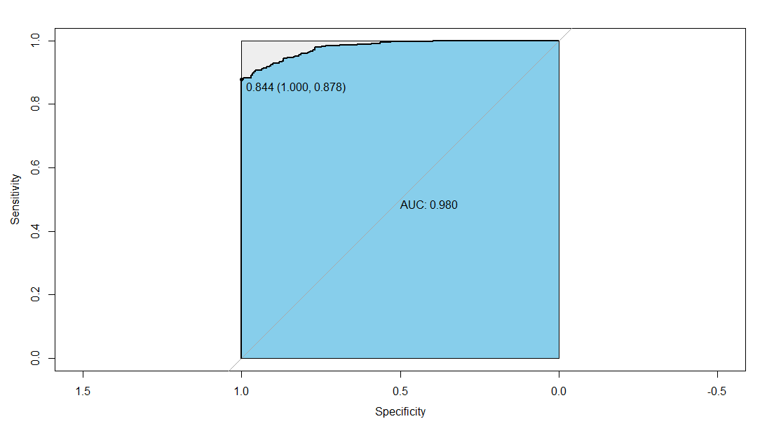
ROC曲线进行模型评估，找出训练集最优阈值

说明：训练集最优阈值是0.844，TPR=0.878，FPR=1，AUC=0.980

> pre_logistic_train<-predict(step_logistic,train_data,type="response")

> library(pROC)

> fit_roc_train<-roc(train_data$是否流失,pre_logistic_train)

> plot(fit_roc_train,print.auc=TRUE,auc.polygon=TRUE,max.auc.polygon=TRUE,auc.polygon.col="skyblue",print.thres=TRUE)

> ##说明：最优阈值是0.844，TPR=0.878，FPR=1，AUC=0.980

> pre_logistic_train=ifelse(pre_logistic_train>0.844,1,0)

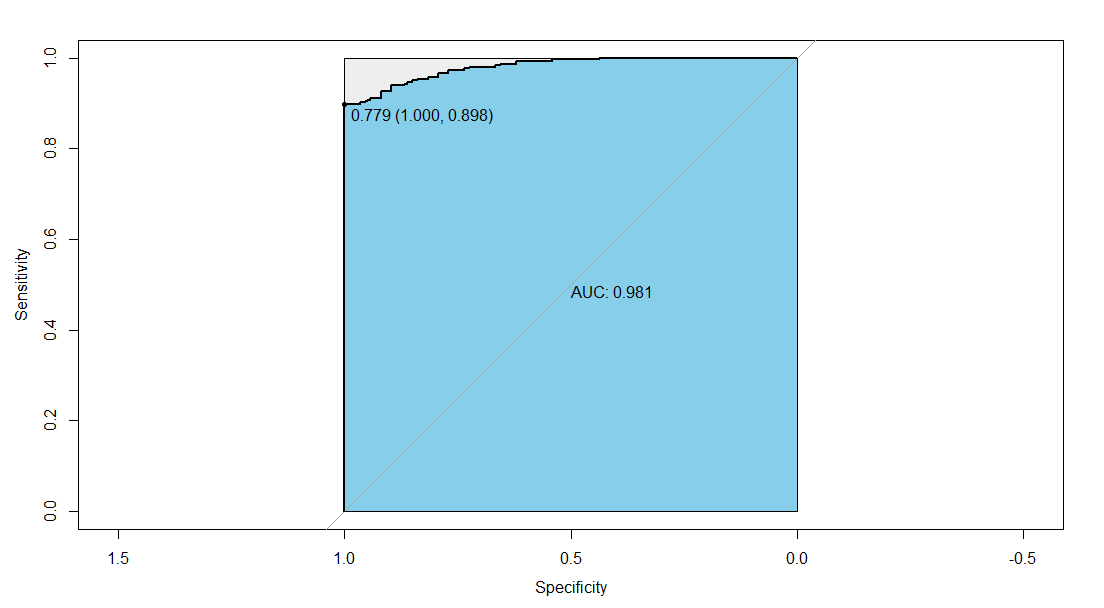
ROC曲线进行模型评估，找出测试集最优阈值

说明：测试集最优阈值是0.779，TPR=0.898，FPR=1，AUC=0.981

> pre_logistic_test<-predict(step_logistic,test_data,type="response")

> library(pROC)

> fit_roc_test<-roc(test_data$是否流失,pre_logistic_test)

> plot(fit_roc_test,print.auc=TRUE,auc.polygon=TRUE,max.auc.polygon=TRUE,auc.polygon.col="skyblue",print.thres=TRUE)

> pre_logistic_test=ifelse(pre_logistic_test>0.779,1,0)

##所有模型训练集及测试集预测结果比较

说明：各模型的不管是train_data还是test_data，Accuracy都在90%以上，效果非常好。训练集中，随机森林的预测效果竟达到100%，其中：

c5.0:train-test=0.935-0.923=0.012

randomForest:train-test=1-0.921=0.079

nnet:train-test=0.923-0.921=0.02

logistic:train-test=0.905-0.921=-0.016

前三个的训练集效果均好与测试集，最后训练集效果反而小于测试集，但是除了随机森林前后预测效果差距比较大之外，其余的差距并不大。需要考虑随机森林是否过拟合。

> name<-c("t_c5.0","t_randomForest","t_nnet","t_logistic")

> test_table=train_table<-list()

> compare_test=compare_train<-as.data.frame(matrix(rep(0,20),nrow = 4))

> rownames(compare_test)=rownames(compare_train)<-name

> colnames(compare_test)=colnames(compare_train)<-c("Accuracy","Kappa","Sensitivity","Specificity","Precision" )

> for(i in 1:4){

+   t_train<-confusionMatrix(switch(i,pre_c5.0_train,pre_randomForest_train,pre_nnet_train,pre_logistic_train),train_data$是否流失)

+   t_test<-confusionMatrix(switch(i,pre_c5.0_test,pre_randomForest_test,pre_nnet_test,pre_logistic_test),test_data$是否流失)

+   compare_train[i,]<-round((t(c(t_train$overall[1:2],t_train$byClass[c(1,2,5)]))),3)

+   compare_test[i,]<-round((t(c(t_test$overall[1:2],t_test$byClass[c(1,2,5)]))),3)

+   train_table[[i]]<-t_train$table

+   test_table[[i]]<-t_test$table

+ }

> compare_train;compare_test

               Accuracy Kappa Sensitivity Specificity Precision

t_c5.0            0.935 0.817       0.897       0.945     0.824

t_randomForest    1.000 1.000       1.000       1.000     1.000

t_nnet            0.923 0.767       0.770       0.966     0.867

t_logistic        0.905 0.762       1.000       0.878     0.701

               Accuracy Kappa Sensitivity Specificity Precision

t_c5.0            0.923 0.782       0.851       0.944     0.813

t_randomForest    0.921 0.776       0.851       0.941     0.804

t_nnet            0.921 0.758       0.747       0.970     0.878

t_logistic        0.921 0.797       1.000       0.898     0.737

> names(train_table)=names(test_table)<-name

> train_table;test_table

$t_c5.0

          Reference

Prediction   0   1

         0 183  39

         1  21 674



$t_randomForest

          Reference

Prediction   0   1

         0 204   0

         1   0 713



$t_nnet

          Reference

Prediction   0   1

         0 157  24

         1  47 689



$t_logistic

          Reference

Prediction   0   1

         0 204  87

         1   0 626



$t_c5.0

          Reference

Prediction   0   1

         0  74  17

         1  13 288



$t_randomForest

          Reference

Prediction   0   1

         0  74  18

         1  13 287



$t_nnet

          Reference

Prediction   0   1

         0  65   9

         1  22 296



$t_logistic

          Reference

Prediction   0   1

         0  87  31

         1   0 274

#随机森林过拟合诊断（以下均为谢老师书中的R代码）

随机森林默认决策树数目为500，接着分别计算不同数目下的误差率。

> n=500

> nerr_train=nerr_test<-rep(0,n)

> for(i in 1:n){

+   fit<-randomForest(是否流失~.,data=train_data,mtry=6,ntree=i)

+   train<-predict(fit,train_data,type="class")

+   test<-predict(fit,test_data,type="class")

+   nerr_train[i]<-sum(train_data$是否流失!=train)/nrow(train_data)

+   nerr_test[i]<-sum(test_data$是否流失!=test)/nrow(test_data)

+ }

> plot(1:n,nerr_train,type = "l",ylim = c(min(nerr_train,nerr_test),max(nerr_train,nerr_test)),xlab="数的数目",ylab="误差率",lty=1,col=1)

> lines(1:n,nerr_test,lty=2,col=2)

> legend("right",lty=1:2,col=1:2,legend =c("训练集","测试集"),bty="n",cex=0.8)

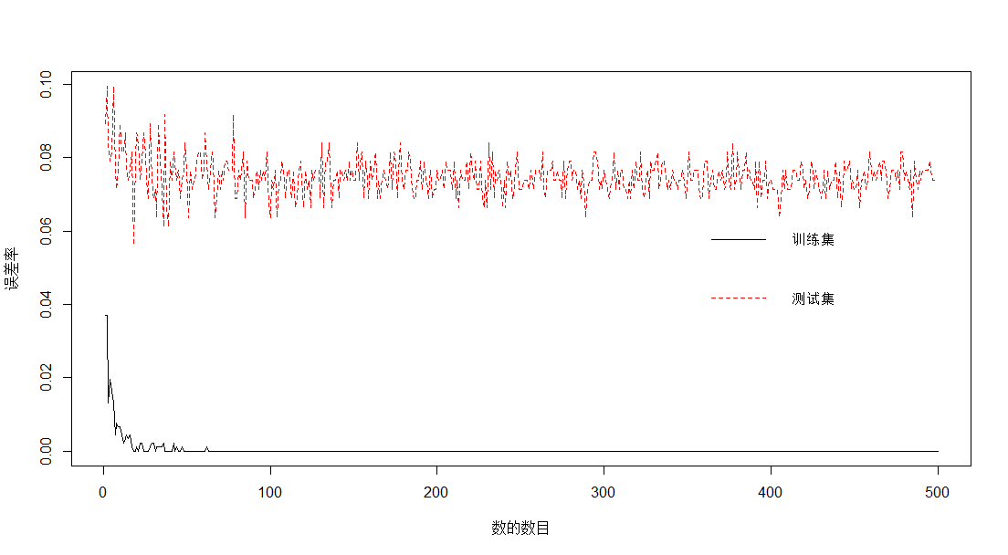
说明：图形给出了随机森林的ntree取不同数值时，训练集与测试集的误差大小，随着取值不断增大，训练集误差在0处稳定，测试集误差波动幅度不断减小，在0.075左右上下波动。可见，随机森林对结果的预测并非过拟合。