这一期主要应用python和R 这2种工具对某真实信贷数据进行分析，通过数据的读取、清洗、探索、模型构建等，比较2种方法在机器学习数据科学上的实现。python实现部分借鉴了KUNAL JAIN 在Analytics Vidhya中的一篇文章《A Complete Tutorial to Learn Data Science with Python from Scratch》（下面有原文链接）。

目 录

1  数据科学探索（python 与 R 的比较）

1.1  数据读取

1.1.1  Python

1.1.2  R

1.2  数据描述

1.2.1  python

1.2.2  R

1.3  数据处理

1.3.1  python

1.3.2  R

1.4  建立预测模型

1.4.1  python

1.4.2  R

1.5  Logistic

1.5.1  python

1.5.2  R

1.6  决策树

1.6.1  python

1.6.2  R

1.7  随机森林

1.7.1  python

1.7.2  R

1 数据科学探索（python 与 R 的比较）

        首次尝试使用jupyter notebook来实现python 和 R，感觉在R的部分兼容性方面还是与rmarkdown有些差距。也许是还不熟悉的原因吧。如何在jupyter中跑R 可以查看[Jupyter and conda for R](http://www.tuicool.com/articles/nuaiEnF) 这篇文章.

    我们分别从数据科学的主要流程来讨论Python与R 的数据实现。

1.1 数据读取

1.1.1 Python

   在python中运用jupyter notebook绘制图形，需要“%matplotlib inline”在代码开头说明。载入相应的库，主要包括numpy、pandas、matplotlib等。python与R一般的操作比较，直接比较代码即可。

%matplotlib inline

import pandas as pd

import numpy as np

import matplotlib.pyplot as plt

df = pd.read_csv("C:/Users/HP/Desktop/train.csv")

df.head()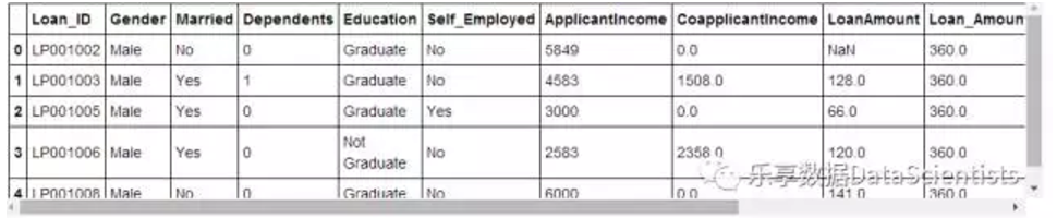

df.describe()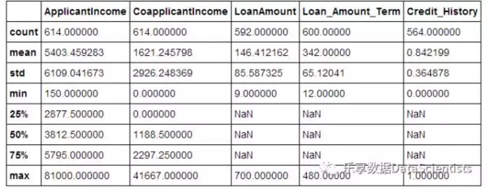

1.1.2 R

    在jupyter中跑R，除安装好R的驱动kernel外，下载并加载包，需要先指定mirror（本人版本如此，求高人指点）。运用psych包中的describe函数可获得类似Python效果。

#设置mirror
local({r <- getOption("repos")r["CRAN"] <- "http://mirrors.xmu.edu.cn/CRAN/"options(repos=r)})

library(ggplot2)
library(dplyr)
library(psych)
library(Hmisc)

train <- read.csv("C:/Users/HP/Desktop/train.csv")

head(train)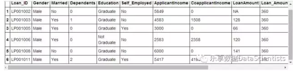

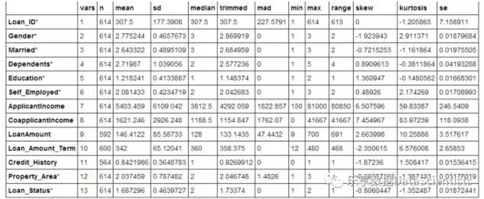
data.frame(psych::describe(train))

1.2数据描述

        主要包括对计量资料和分类变量的分布进行绘图描述。python主要运用到matplotlib库，R主要运用到ggplot2包。从数据描述及绘图效果来看，python绘制一般图形相对简单，但R运用ggplot图层语法绘图感觉更易理解和操作。

1.2.1 python

#查看申请人地域分布
df['Property_Area'].value_counts()

Semiurban    233

Urban        202

Rural        179

Name: Property_Area, dtype: int64

#查看申请人收入分布情况
df['ApplicantIncome'].hist(bins=50)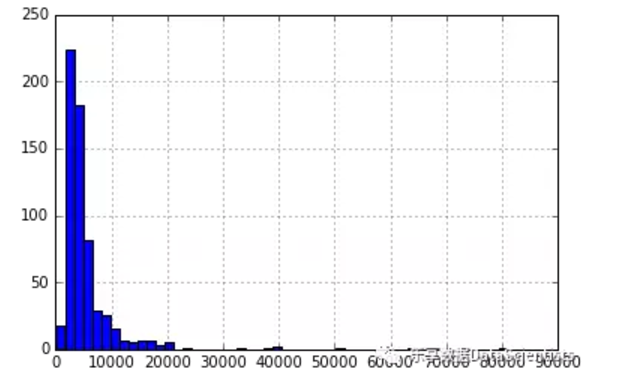

#按教育情况分类，查看收入情况
df.boxplot(column='ApplicantIncome', by = 'Education')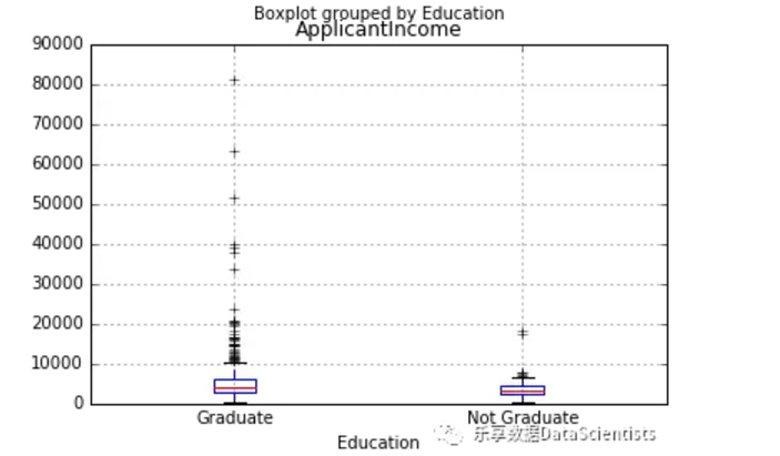

#查看申请人信用历史分布并绘图
temp1 = df['Credit_History'].value_counts(ascending=True)
temp2 = df.pivot_table(values='Loan_Status', index=['Credit_History'],aggfunc=lambda x: x.map({'Y':1,"N":0}).mean())
print 'Frequency Table for Credit History:'print temp1



print '\nProbility of getting loan for each Credit History class:'print temp2

Frequency Table for Credit History:

0.0     89

1.0    475

Name: Credit_History, dtype: int64



Probility of getting loan for each Credit History class:

Credit_History

0.0    0.078652

1.0    0.795789

Name: Loan_Status, dtype: float64

import matplotlib.pyplot as plt

fig = plt.figure(figsize=(8,4))
ax1 = fig.add_subplot(121)ax1.set_xlabel('Credit_History')
ax1.set_ylabel('Count of Applicants')
ax1.set_title('Applicants by Credit_History')
temp1.plot(kind= 'bar')

ax2 = fig.add_subplot(122)
temp2.plot(kind = 'bar')
ax2.set_xlabel('credit_history')
ax2.set_ylabel('probability of getting loan')
ax2.set_title('probability of getting loan by credit history')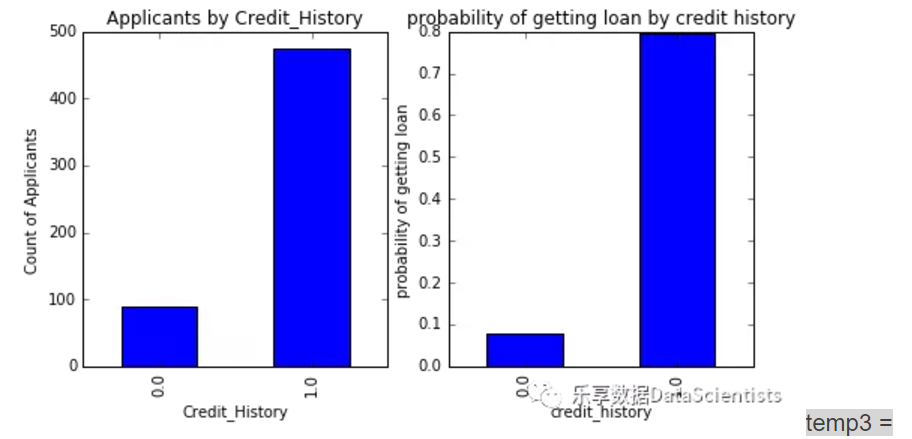

pd.crosstab(df['Credit_History'], df['Loan_Status'])

temp3.plot(kind='bar', stacked=True, color=['red','blue'],grid=False)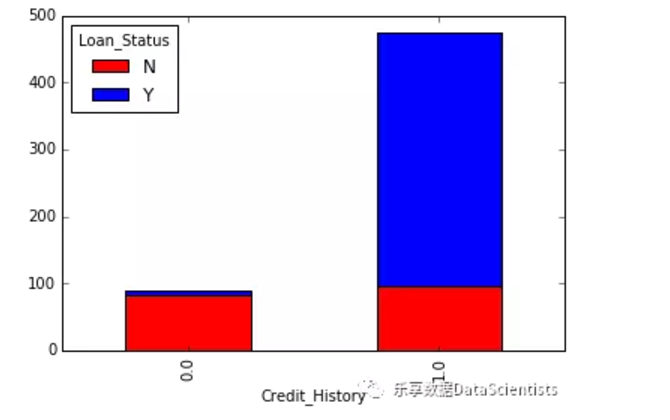

1.2.2 R

#申请人地域分布
table(train$Property_Area)

Rural Semiurban     Urban 

  179       233       202 

#申请人收入分布情况
ggplot(data=train, aes(x=ApplicantIncome)) + geom_histogram(bins = 50, fill = "blue")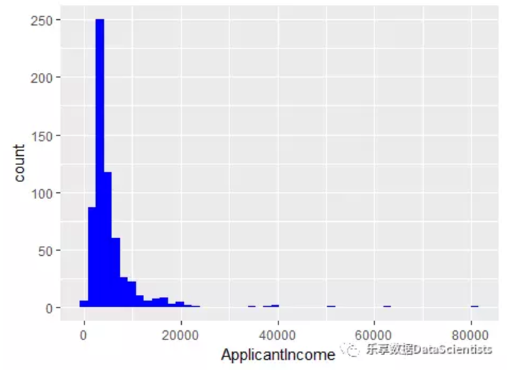

ggplot(data=train, aes(x=Education, y=ApplicantIncome)) + geom_boxplot()

1.3 数据处理

       数据处理主要包括以下方面：

1. 缺失值处理

2. 极值处理

        对数据的处理，这里缺失值填补只运用了最简单的平均数或众数替换，数据变换也只进行相对简单的log变换等。感觉R的dplyr包管道操作在数据处理方面比python更胜一筹。

1.3.1 python

# 检测缺失值
df.apply(lambda x: sum(x.isnull()), axis = 0)

Loan_ID               0

Gender               13

Married               3

Dependents           15

Education             0

Self_Employed        32

ApplicantIncome       0

CoapplicantIncome     0

LoanAmount           22

Loan_Amount_Term     14

Credit_History       50

Property_Area         0

Loan_Status           0

dtype: int64

#计量资料用均值、计数资料用众数填补
df['LoanAmount'].fillna(df['LoanAmount'].mean(),inplace=True)

#查看分布
df['Self_Employed'].value_counts()
df['Credit_History'].value_counts()
df['Gender'].value_counts() 
df['Loan_Amount_Term'].value_counts()
df['Dependents'].value_counts()
df['Married'].value_counts()

Yes    398

No     213

Name: Married, dtype: int64

df['Loan_Amount_Term'].fillna(360.0,inplace=True)

df['Gender'].fillna(2,inplace=True)

df['Credit_History'].fillna(1.0,inplace=True)df['Dependents'].fillna(0,inplace=True)

table = df.pivot_table(values='LoanAmount',index='Self_Employed',columns='Education',aggfunc=np.median)print(table)

Education      Graduate  Not Graduate

Self_Employed                        

NO                126.5         123.0

No                132.0         115.0

Yes               152.0         130.0

df['Self_Employed'].fillna('NO',inplace=True)df['Married'].fillna('YES',inplace=True)

#最后查看填补结果
df.apply(lambda x: sum(x.isnull()), axis = 0)

Loan_ID              0

Gender               0

Married              0

Dependents           0

Education            0

Self_Employed        0

ApplicantIncome      0

CoapplicantIncome    0

LoanAmount           0

Loan_Amount_Term     0

Credit_History       0

Property_Area        0

Loan_Status          0

dtype: int64

#数据变换#转换为收入log值
df['LoanAmount_log'] = np.log(df['LoanAmount'])df['LoanAmount_log'].hist(bins=20)

df['TotalIncome'] = df['ApplicantIncome'] + df['CoapplicantIncome']
df['TotalIncome_log'] = np.log(df['TotalIncome'])df['LoanAmount_log'].hist(bins=20)

1.3.2 R

#查看缺失情况
pMiss <- function(x) {

    sum(is.na(x))/length(x)*100 }
apply(train, 2, pMiss)

      Loan_ID            Gender           Married        Dependents         Education 

     0.000000          0.000000          0.000000          0.000000          0.000000 

Self_Employed   ApplicantIncome CoapplicantIncome        LoanAmount  Loan_Amount_Term 

     0.000000          0.000000          0.000000          3.583062          2.280130 

library(Hmisc)
train$LoanAmount <- Hmisc::impute(train$LoanAmount, mean)

train$Loan_Amount_Term <- impute(train$Loan_Amount_Term, 360.0)
train$Credit_History <- impute(train$Credit_History, 1.0)
train$Self_Employed <- impute(train$Self_Employed, "NO")
train$Married <- impute(train$Married, "YES")
train$Gender <- impute(train$Gender, 2)

#数据变换#转换为收入log值
library(dplyr)
train = mutate(train, LoanAmount_log = log(LoanAmount), TotalIncome = ApplicantIncome + CoapplicantIncome,TotalIncome_log =log(TotalIncome))
apply(train, 2, pMiss)

      Loan_ID            Gender           Married        Dependents         Education 

            0                 0                 0                 0                 0 

Self_Employed   ApplicantIncome CoapplicantIncome        LoanAmount  Loan_Amount_Term 

            0                 0                 0                 0                 0 

1.4 建立预测模型

      在建立预测模型方面，分布建立logistic回归、决策树、随机森林并加以比较和改善。从代码编辑上看，python通过sklearn库构建预测模型函数，实现建立模型的打包处理，比R 分别调用不同的包进行模型模拟有更大的优势，值得学习和借鉴。

1.4.1 python

#转变所有的分类变量为数值变量
from sklearn.preprocessing import LabelEncoder

var_mod = ['Gender','Married','Dependents','Education','Self_Employed','Property_Area','Loan_Status']le = LabelEncoder()for i in var_mod:

    df[i] = le.fit_transform(df[i])df.dtypes

Loan_ID               object

Gender                 int64

Married                int64

Dependents             int64

Education              int64

Self_Employed          int64

ApplicantIncome        int64

CoapplicantIncome    float64

LoanAmount           float64

Loan_Amount_Term     float64

Credit_History       float64

Property_Area          int64

Loan_Status            int64

LoanAmount_log       float64

TotalIncome          float64

TotalIncome_log      float64

dtype: object

#载入sklearn库，选择相应的操作。

from sklearn.cross_validation import KFold   #For K-fold cross validationfrom sklearn.ensemble import RandomForestClassifier

from sklearn.tree import DecisionTreeClassifier, export_graphviz

from sklearn import metrics#Generic function for making a classification model and accessing performance:def classification_model(model, data, predictors, outcome):

  #拟合模型

  model.fit(data[predictors],data[outcome])

  

  #在训练集上预测模型

  predictions = model.predict(data[predictors])

  

  #打印模型准确性

  accuracy = metrics.accuracy_score(predictions,data[outcome])

  print "Accuracy : %s" % "{0:.3%}".format(accuracy) 
#完成5折交叉验证
kf = KFold(data.shape[0], n_folds=5)  
error = []  
for train, test in kf:      
  train_predictors = (data[predictors].iloc[train,:])        
  train_target = data[outcome].iloc[train]        
  model.fit(train_predictors, train_target)   #拟合模型       
  error.append(model.score(data[predictors].iloc[test,:], data[outcome].iloc[test]))   
print "Cross-Validation Score : %s" % "{0:.3%}".format(np.mean(error))



#模型最终拟合

model.fit(data[predictors],data[outcome])

1.4.2 R

library(rpart)
library(e1071)
library(rpart.plot)
library(caret)
library(Metrics)

test <- read.csv("C:/Users/HP/Desktop/test.csv")

1.5 Logistic

1.5.1 python

outcome_var = 'Loan_Status'model = LogisticRegression()predictor_var = ['Credit_History']classification_model(model, df,predictor_var,outcome_var)

Accuracy : 80.945%

Cross-Validation Score : 80.946%

1.5.2 R

#设置控制参数
fitControl <- trainControl(method = "cv", number = 5)
#拟合模型
logistic_model <- train(Loan_Status ~., data= train, method = "glmnet", trControl = fitControl, family="binormal")
print(logistic_model)

#选择最优模型logistic_model <- train(Loan_Status ~., data= train, method = "glmnet", trControl = fitControl, family="binormal")
#模型预测logistic_predict <- predict(logistic_model, newdata= test,type = "vector")

#模型评价
confusionMatrix(train$Loan_Status, logistic_model)

1.6 决策树

1.6.1 python

model = DecisionTreeClassifier()predictor_var = ['Credit_History','Gender','Married','Education']classification_model(model, df,predictor_var,outcome_var)

Accuracy : 80.945%

Cross-Validation Score : 80.946%

1.6.2 R

#设置控制参数
fitControl <- trainControl(method = "cv", number = 5)cartGrid <- expand.grid(.cp=(1:50)*0.01)
#拟合模型
tree_model <- train(Loan_Status ~Credit_History+Gender+Married+Education, data= train, method = "rpart", trControl = fitControl, tuneGrid = cartGrid)
print(tree_model)

#选择最优决策树模型main_tree <- rpart(Loan_Status ~., data= train, control = rpart.control(cp=0.36))

#绘制决策树prp(main_tree)

#模型预测pre_score <- predict(main_tree,type = "vector")#模型评价xtabs(~ pre_score + train$Loan_Status)

1.7 随机森林

1.7.1 python

#随机森林model = RandomForestClassifier(n_estimators=100)predictor_var = ['Gender', 'Married', 'Dependents', 'Education',

       'Self_Employed', 'Loan_Amount_Term', 'Credit_History', 'Property_Area']classification_model(model, df,predictor_var,outcome_var)

Accuracy : 87.296%

Cross-Validation Score : 76.549%

#变量重要性得分
featimp = pd.Series(model.feature_importances_, index=predictor_var).sort_values(ascending=False)
print featimp

Credit_History      0.427036

Dependents          0.142901

Property_Area       0.102788

Loan_Amount_Term    0.100776

Self_Employed       0.077128

Gender              0.055985

Education           0.048056

Married             0.045331

dtype: float64

model = RandomForestClassifier(n_estimators=25, min_samples_split=25, max_depth=7, max_features=1)
predictor_var = ['Credit_History','Dependents','Property_Area']classification_model(model, df,predictor_var,outcome_var)

Accuracy : 80.945%

Cross-Validation Score : 80.458%

1.7.2 R

library(randomForest)

#设置参数
control <- trainControl(method = "cv", number = 5)
#随机森林
rf_model <- train(Loan_Status ~Credit_History+Dependents+Property_Area, data= train, method = "parRF",

                 trControl= control, prox = TRUE, allowParallel= TRUE)print(rf_model)

#选择最优决策树
forest_model <- randomForest(Loan_Status ~Credit_History+Dependents+Property_Area, data= train,

                            mtry = 15, ntree = 1000)print(forest_model)

#查看变量重要性排序
varImplot(forest_model)

#模型预测
main_predict <- predict(forest_model, newdata= test,type = "vector")

#模型评价
confusionMatrix(train$Loan_Status, main_predict)

写在文后（此处有雷）：

       由于在jupyter中跑R，有些模型会出现一些莫名的问题和错误，因此R有些代码在jupyter中并不能跑成功。本人也在抓紧找出原因并解决，如出现错误，请各位大侠指正。感激不尽！

”乐享数据“个人公众号，不代表任何团体利益，亦无任何商业目的。任何形式的转载、演绎必须经过公众号联系原作者获得授权，保留一切权力。欢迎关注“乐享数据”。