数据中的离群值往往会扭曲预测结果并影响模型精度，回归模型中离群值的影响尤其大，因此我们需要对其进行检测和处理。

离群值检测的重要性

处理离群值或者极端值并不是数据建模的必要流程，然而，了解它们对预测模型的影响也是大有裨益的。数据分析师们需要自己判断处理离群值的必要性，并结合实际问题选取处理方法。那么，检测离群值的重要性体现在哪儿呢？其实，由于离群值的存在，模型的估计和预测可能会有很大的偏差或者变化。我们用汽车数据来说明这个现象。

我将用包含和不含离群值的汽车数据来建立一个简单的线性回归模型，以此阐述离群值的影响。为了更好的区分它的效应，我在原始数据集中人为地加入了极端值，然后利用线性归回做预测。

# 给数据集插入离群值

cars1 <- cars[1:30,  ]  # 原始数据

cars_outliers <- data.frame(speed = c(19, 19, 20, 20, 20), 

                            dist = c(190, 186, 210, 220, 218))  # 引入离群值

cars2 <- rbind(cars1, cars_outliers)  # 包含李全职的数据



# 绘制包含离群值的数据建模结果

par(mfrow = c(1, 2))

plot(cars2$speed, cars2$dist, xlim = c(0, 28), ylim=c(0, 230), 

     main = "With Outliers", xlab = "speed", ylab = "dist", 

     pch = "*", col = "red", cex = 2)

abline(lm(dist ~ speed, data = cars2), col = "blue", lwd = 3, lty = 2)



# 绘制原始数据建模加过，留意回归线斜率的变化

plot(cars1$speed, cars1$dist, xlim = c(0, 28), ylim = c(0, 230), 

     main = "Outliers removed \n A much better fit!",

     xlab = "speed", ylab = "dist", pch = "*", col = "red", cex = 2)

abline(lm(dist ~ speed, data = cars1), col = "blue", lwd = 3, lty = 2)

结果如下

留意一下移除离群值后拟合线的斜率变化。如左图所示，如果用包含离群值的数据训练模型，我们预测结果在速度很快的数据上会有很大的误差，因为回归线非常陡峭。

检测离群值

1. 单变量检测法

给定一个连续变量后，离群值可以认为是哪些超出1.5倍四分位距的观测点。四分位距（Inter Quartile Range, a.k.a IQR）是0.25分位数和0.75分位数的差，我们可以通过箱线图来检测离群点，在须轴以外的点就是。

url <- "http://rstatistics.net/wp-content/uploads/2015/09/ozone.csv"  

# 备用数据源: https://raw.githubusercontent.com/selva86/datasets/master/ozone.csv

inputData <- read.csv(url)  # 导入数据



outlier_values <- boxplot.stats(inputData$pressure_height)$out  # outlier values.

boxplot(inputData$pressure_height, main="Pressure Height", boxwex=0.1)

mtext(paste("Outliers: ", paste(outlier_values, collapse=", ")), cex=0.6)

2. 双变量检测法

如果有两个变量X和Y，X是分类变量而Y是连续变量，可以绘制在X的不同类别上Y的箱线图来检测离群值。

url <- "http://rstatistics.net/wp-content/uploads/2015/09/ozone.csv"

ozone <- read.csv(url)



# Month和Day_of_Week是分类变量

boxplot(ozone_reading ~ Month, data=ozone, main="Ozone reading across months")  # 有明确的模式

boxplot(ozone_reading ~ Day_of_week, data=ozone, main="Ozone reading for days of week")  # this may not be significant, as day of week variable is a subset of the month var.

箱线图如下：

上图我们发现每个月的ozone_reading数据有明显变化，但在周内每天的区别并不明显。每一个类别中，在箱线图须轴以外的店就是离群值。

如果X和Y都是连续变量，我们可以将X离散化

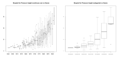
boxplot(ozone_reading ~ pressure_height, data=ozone, 

        main="Boxplot for Pressure height (continuos var) vs Ozone")

boxplot(ozone_reading ~ cut(pressure_height, pretty(inputData$pressure_height)), 

        data=ozone, main="Boxplot for Pressure height (categorial) vs Ozone", cex.axis=0.5)

结果如下

离散化处理后，你会发现被判定为离群值的点更少，并且ozone_reading随着pressure_height的增加而变化的趋势愈发明确了。

3. 多元模型检测法

仅凭一个特征就判定一个观测值是离群点可能并不科学。利用多个特征的信息来判断个体是否是离群值会更好，这就需要使用Cook距离。

Cook距离可以衡量一个给定的回归模型是否只受单个变量X的影响。Cook距离会极端每一个数据点对预测结果的影响。对于每个观测i，Cook距离会衡量包含i与不包含i时，Y的拟合值的变化，这样我们就知道了i对拟合结果的影响了。

观测i的Cook距离计算公式如下：

其中：

是使用所有观测计算的第j个y的拟合值

是使用除观测i外所有观测计算的第j个y的拟合值

是均方误差

是回归模型的系数个数

mod <- lm(ozone_reading ~ ., data=ozone)

cooksd <- cooks.distance(mod)

影响评估

一般来说，如果某个观测的Cook距离比平均距离大4倍，我们就可以认为这个点是离群点，当然这不是一个非常死板的判定条件。

plot(cooksd, pch="*", cex=2, main="Influential Obs by Cooks distance")  # 绘制Cook距离

abline(h = 4*mean(cooksd, na.rm=T), col="red")  # 添加决策线

text(x=1:length(cooksd)+1, y=cooksd, labels=ifelse(cooksd>4*mean(cooksd, na.rm=T),names(cooksd),""), col="red")  # 添加标签

结果如下：

现在让我们从原始数据集中找出那些影响力特别大的观测点吧。如果你把它们逐一挑出来了，你就能发现为何它们会有这么大的影响力了——这些观测的在某些变量上的取值过于极端了。

influential  4*mean(cooksd, na.rm=T))])  # 有影响力的观测值行标

head(ozone[influential, ])  # 列出这些观测

#>     Month Day_of_month Day_of_week ozone_reading pressure_height Wind_speed Humidity

#> 19      1           19           1          4.07            5680          5       73

#> 23      1           23           5          4.90            5700          5       59

#> 58      2           27           5         22.89            5740          3       47

#> 133     5           12           3         33.04            5880          3       80

#> 135     5           14           5         31.15            5850          4       76

#> 149     5           28           5          4.82            5750          3       76

#>     Temperature_Sandburg Temperature_ElMonte Inversion_base_height Pressure_gradient

#> 19                    52               56.48                   393               -68

#> 23                    69               51.08                  3044                18

#> 58                    53               58.82                   885                -4

#> 133                   80               73.04                   436                 0

#> 135                   78               71.24                  1181                50

#> 149                   65               51.08                  3644                86

#>     Inversion_temperature Visibility

#> 19                  69.80         10

#> 23                  52.88        150

#> 58                  67.10         80

#> 133                 86.36         40

#> 135                 79.88         17

#> 149                 59.36         70

让我们看看前6个观测来看看为什么这些观测富有影响力吧。

• 第58， 133， 135行的ozone_reading值非常大
• 第23， 135， 149行的Inversion_bzase_height值非常大
• 第19行有非常低的Pressure_gradient

离群值检验

car包中的outlierTest函数可以返回指定模型中影响力最大的观测值。

car::outlierTest(mod)

#> No Studentized residuals with Bonferonni p  Largest |rstudent|:

#>     rstudent unadjusted p-value Bonferonni p

#> 243 3.045756          0.0026525      0.53845

0utliners包

outliers包提供了几个有用的函数来系统地检测出离群值。其中一些函数既便利又好上手，特别是outliers()函数和scores()函数。

outliers()会返回和平均值相比较后最极端的观测，如果你给定参数opposite=TRUE，它会返回位于另一端的观测。

set.seed(1234)

y=rnorm(100)

outlier(y)

#> [1] 2.548991

outlier(y,opposite=TRUE)

#> [1] -2.345698

dim(y) <- c(20,5)  # convert it to a matrix

outlier(y)

#> [1] 2.415835 1.102298 1.647817 2.548991 2.121117

outlier(y,opposite=TRUE)

#> [1] -2.345698 -2.180040 -1.806031 -1.390701 -1.372302

scores()函数有两大功能。一是计算规范化得分，诸如z得分，t得分，chisq得分等。它还可以基于上述的得分值，返回那些得分在相应分布百分位数之外的观测值。

set.seed(1234)

x = rnorm(10)

scores(x)  # z得分 => (x-mean)/sd

scores(x, type="chisq")  # chisq得分 => (x - mean(x))^2/var(x)

#> [1] 0.68458034 0.44007451 2.17210689 3.88421971 0.66539631  . . .

scores(x, type="t")  # t得分

scores(x, type="chisq", prob=0.9)  # 是否超过chisq分布的0.9分位数

#> [1] FALSE FALSE FALSE  TRUE FALSE FALSE FALSE FALSE FALSE FALSE

scores(x, type="chisq", prob=0.95)  # 0.95分位数

scores(x, type="z", prob=0.95)  # 基于z得分判定

scores(x, type="t", prob=0.95)  # 大家都懂，我懒得翻译了

离群值处理

在寻找到离群值之后，你需要根据处理的实际问题来对它们进行处理，常用方法如下：

1. 插值

使用均值/中位数/众数插值，这个方法在缺失值的处理邻领域已被广泛应用。另一种稳健的做法是使用链式方程进行多元插值。

2. 封顶

对于那些取值超过1.5倍四分位距的数值，可以分别用该变量5%和95%的分位数替代原数据，下方代码可以实现该过程：

x <- ozone$pressure_height

qnt <- quantile(x, probs=c(.25, .75), na.rm = T)

caps <- quantile(x, probs=c(.05, .95), na.rm = T)

H <- 1.5 * IQR(x, na.rm = T)

x[x < (qnt[1] - H)]  (qnt[2] + H)] <- caps[2]

译者注：该方法和数据预处理中的缩尾（winsorize）处理基本一致，和数理统计中的m统计量思想也类似。

注:原文刊载于datascience+网站

链接:Outlier detection and treatment with R