
前言
接触金融时间并不太长,对我来说第一个操作的业务,就是逆回购。逆回购对于大部分人来说,都是一个新鲜词,就算是炒股多年的玩家,可能也是在2013年6月份发生银行缺钱的事件之后才了解的。隔夜的银行间拆借利率达到了30%,简单来说银行缺钱了!各种机构 分分出售股票,债券,兑换成现金借给应银行。个人用户也都取出存款,通过逆回购,把钱借给银行。30%的利率,让所有人在那一周都为之兴奋,只有银行在惶恐。
目录
- 逆回购简介
- 历史数据模型
- 通过用RHive提取数据
- 简单策略实现
1. 逆回购简介
债券回购的含义
债券质押式回购简单地说就是交易双方以债券为质押品的一种短期资金借贷行为。其中债券持有人(正回购方)将债券质押而获得资金使用权,到约定的时间还本并支付一定的利息,从而“赎回”债券。而资金持有人(逆回购方)就是正回购方的交易对手。在实际交易中债券是质押给了第三方即中国结算公司,这样交易双方否更加安全、便捷。
可回购的债券
所有的国债、绝大部分企业债、公司债和分离债的纯债都可用于债券回购交易。沪深交易所每周都会公布可回购债券的折算率,上面没有但可交易的品种就是不可回购的债券。折算率简单说,就是把债券质押时,交易所按债券面值给出的可质押的比率。
现在交易的回购品种
我们仅列出个人投资者经常参与的公司债(包括企业债等)回购品种。
上海证券交易所可交易的质押式回购(括弧中为交易代码)分为1日(204001)、2日(204002)、3日(204003)、4日(204004)、7日(204007)、14日(204014)、28日(204028)、91日(204091)、182日(204182)共9个品种。深圳交易所按回购期限分为分为1日(131810)、2日(131811)、3日(131800)、7日(131801)共4个品种。其中经常交易的只有沪深1日和7日四个品种,并且沪市的日均交易量又远远大于深市的交易量。
以上逆回购定义摘自:http://finance.sina.com.cn/money/bond/20121016/180713385513.shtml
2. 历史数据模型
Hive中的表结构:
rhive.desc.table('t_reverse_repurchase')

    col_name data_type

1  tradedate    string

2  tradetime    string

3 securityid    string

4     bidpx1    double

5   bidsize1    double

6   offerpx1    double

7 offersize1    double
tradedate:交易日期
tradetime:交易时间
securityid:股票ID
bidpx1:买一
bidsize1:买一交易量
offerpx1:卖一
bidsize1:卖一交易量
3. 通过用RHive提取数据
登陆c1服务器,打开R的客户端。
#装载RHive

library(RHive)


#初始化

rhive.init()


#连接到Hive集群

> rhive.connect("c1.wtmart.com")

SLF4J: Class path contains multiple SLF4J bindings.

SLF4J: Found binding in [jar:file:/home/cos/toolkit/hive-0.9.0/lib/slf4j-log4j12-1.6.1.jar!/org/slf4j/impl/StaticLoggerBinder.class]

SLF4J: Found binding in [jar:file:/home/cos/toolkit/hadoop-1.0.3/lib/slf4j-log4j12-1.4.3.jar!/org/slf4j/impl/StaticLoggerBinder.class]

SLF4J: See http://www.slf4j.org/codes.html#multiple_bindings for an explanation.


#查看当前的表

> rhive.list.tables()

              tab_name

1            t_hft_day   //历史数据表

2            t_hft_tmp   //临时表

4 t_reverse_repurchase   //逆回购表
查看所有股票历史数据分片:测试数据从20130627–20130726。
> rhive.query("SHOW PARTITIONS t_hft_day");

            partition

1  tradedate=20130627

2  tradedate=20130628

3  tradedate=20130701

4  tradedate=20130702

5  tradedate=20130703

6  tradedate=20130704

7  tradedate=20130705

8  tradedate=20130708

9  tradedate=20130709

10 tradedate=20130710

11 tradedate=20130712

12 tradedate=20130715

13 tradedate=20130716

14 tradedate=20130719

15 tradedate=20130722

16 tradedate=20130723

17 tradedate=20130724

18 tradedate=20130725

19 tradedate=20130726
分为提取”上交所一天逆回购”(204001),和”深交所一天逆回购”(131810),从7月22日至7月26日的一周数据。
> rhive.drop.table("t_reverse_repurchase")

> rhive.query("CREATE TABLE t_reverse_repurchase AS SELECT tradedate,tradetime,securityid,bidpx1,bidsize1,offerpx1,offersize1 FROM t_hft_day where tradedate>=20130722 and tradedate<=20130726 and securityid in (131810,204001)");
查看数据结果集
> rhive.query("SELECT securityid,count(1) FROM t_reverse_repurchase group by securityid");

  securityid  X_c1

1     131810 17061

2     204001 12441
加载到R的内存中。
> bidpx1<-rhive.query("SELECT securityid,concat(tradedate,tradetime) as tradetime,bidpx1 FROM t_reverse_repurchase");


#查看记录条数

> nrow(bidpx1)

[1] 29502


#查看数据

> head(bidpx1)

  securityid      tradetime bidpx1

1     131810 20130724145004  2.620

2     131810 20130724145101  2.860

3     131810 20130724145128  2.850

4     131810 20130724145143  2.603

5     131810 20130724144831  2.890

6     131810 20130724145222  2.600
用ggplot2做数据可视化
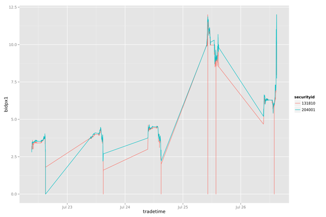
一周数据的走势
library(ggplot2)

g<-ggplot(data=bidpx1, aes(x=as.POSIXct(tradetime,format="%Y%m%d%H%M%S"), y=bidpx1))

g<-g+geom_line(aes(group=securityid,colour=securityid))

g<-g+xlab('tradetime')+ylab('bidpx1')

ggsave(g,file="01.png",width=12,height=8)
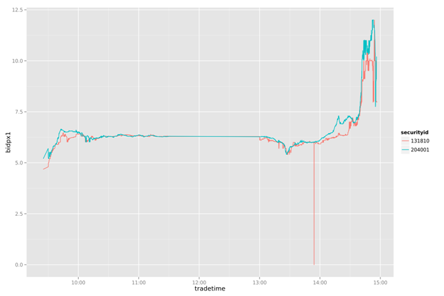
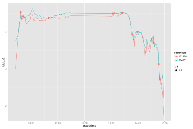
一天数据的走势
bidpx1<-rhive.query("SELECT securityid,concat(tradedate,tradetime) as tradetime,bidpx1 FROM t_reverse_repurchase WHERE tradedate=20130726");

g<-ggplot(data=bidpx1, aes(x=as.POSIXct(tradetime,format="%Y%m%d%H%M%S"), y=bidpx1))

g<-g+geom_line(aes(group=securityid,colour=securityid))

g<-g+xlab('tradetime')+ylab('bidpx1')

ggsave(g,file="02.png",width=12,height=8)
4. 简单策略实现
通过简单的打印出两幅图片的两条曲线,我们可以看到131810一直在追随204001变化,并且大部情况都低于204001。
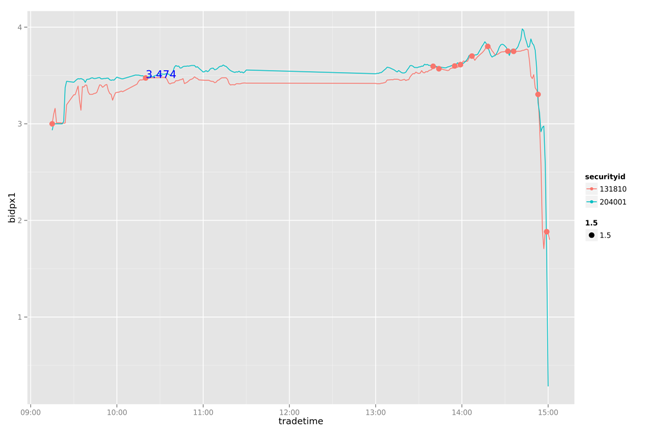
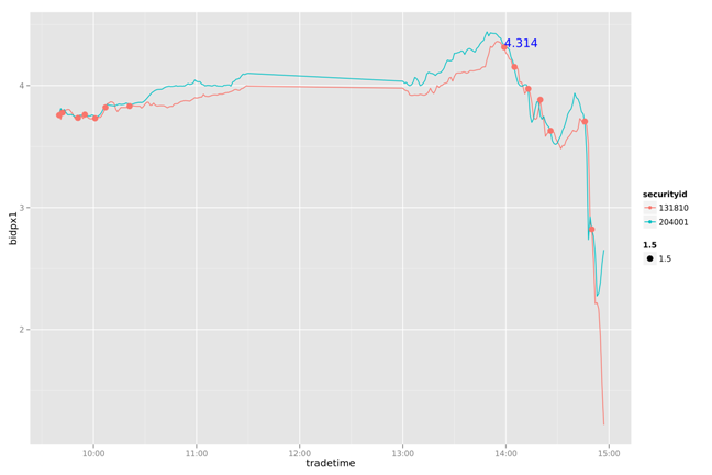
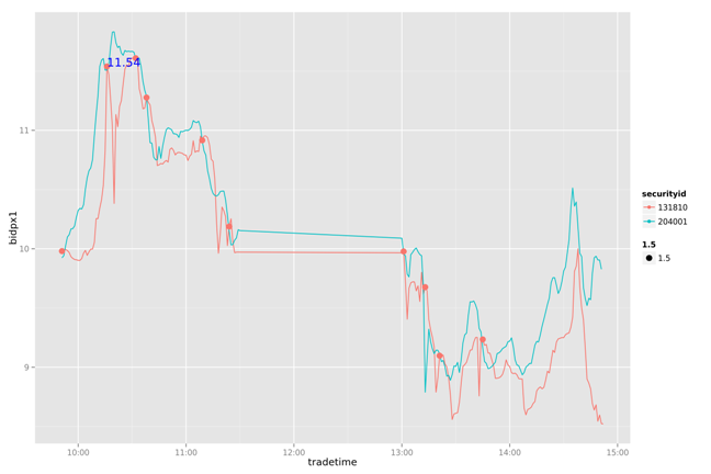
下面做一个简单的策略分析:通过204001变化,判断131810的卖点。
- 把131810和204001按每分钟标准化
- 设置当131810和204001有交点的时候,提取卖出信号
- 当后一个交点的卖一价格大于前一个交点的卖一价格10%以上,做为局部最优的卖出信号点
提取131810,204001的数据,存储在t_reverse_repurchase表中
#登陆R

library(RHive)

rhive.init()

rhive.connect("c1.wtmart.com")


#提取131810,204001的数据

rhive.drop.table("t_reverse_repurchase")

rhive.query("CREATE TABLE t_reverse_repurchase AS SELECT tradedate,tradetime,securityid,bidpx1,bidsize1,offerpx1,offersize1 FROM t_hft_day where securityid in (131810,204001)");


#查看数据集

rhive.query("select count(1),tradedate from t_reverse_repurchase group by tradedate")

   X_c0 tradedate

1  4840  20130627

2  4792  20130628

3  4677  20130701

4  3124  20130702

5  2328  20130703

6  3787  20130704

7  4294  20130705

8  4977  20130708

9  4568  20130709

10 6619  20130710

11 5633  20130712

12 6159  20130715

13 5918  20130716

14 6200  20130719

15 6074  20130722

16 5991  20130723

17 5899  20130724

18 5346  20130725

19 6192  20130726
加载软件包
library(ggplot2)

library(scales)

library(plyr)
获得一天的数据并做ETL
#把一周的数据加载到内存

bidpx1<-rhive.query(paste("SELECT securityid,tradedate,tradetime,bidpx1 FROM t_reverse_repurchase WHERE tradedate>=20130722"));


#加载一天的数据并做ETL

oneDay<-function(date){

  d1<-bidpx1[which(bidpx1$tradedate==date),]

  d1$tradetime2<-round( as.numeric(as.character(d1$tradetime))/100)*100

  d1$tradetime2[which(d1$tradetime2<100000)]<-paste(0,d1$tradetime2[which(d1$tradetime2<100000)],sep="")

  d1$tradetime2[which(d1$tradetime2=='1e+05')]='100000'

  d1$tradetime2[which(d1$tradetime2=='096000')]='100000'

  d1$tradetime2[which(d1$tradetime2=='106000')]='110000'

  d1$tradetime2[which(d1$tradetime2=='126000')]='130000'

  d1$tradetime2[which(d1$tradetime2=='136000')]='140000'

  d1$tradetime2[which(d1$tradetime2=='146000')]='150000'

  d1

}


#通过均值标准化

meanScale<-function(d1){

  ddply(d1, .(securityid,tradetime2), summarize, bidpx1=mean(bidpx1))

}


#找到要分析的点

findPoint<-function(a1,a2){

  #找到所有a1大于a2的点

  bigger_point<-function(a1,a2){

    idx<-c()

    for(i in intersect(a1$tradetime2,a2$tradetime2)){

      i1<-which(a1$tradetime2==i)

      i2<-which(a2$tradetime2==i)

      if(a1$bidpx1[i1]-a2$bidpx1[i2]>=-0.02){

        idx<-c(idx,i1)

      }

    }

    idx

  }


  #去掉连续的索引值

  remove_continuous_point<-function(idx){

    idx[-which(idx-c(NA,rev(rev(idx)[-1]))==1)]

  }


  idx<-bigger_point(a1,a2)

  remove_continuous_point(idx)

}


#发现局部最优卖出点

findOptimize<-function(d3){

  idx2<-which((d3$bidpx1-c(NA,rev(rev(d3$bidpx1)[-1])))/d3$bidpx1>0.1)

  if(length(idx2)<1)

    print("No Optimize point")

  d3[idx2,]

}


#画图查看结果

draw<-function(d2,d3,d4,date,png=FALSE){

  g<-ggplot(data=d2, aes(x=strptime(paste(date,tradetime2,sep=""),format="%Y%m%d%H%M%S"), y=bidpx1))

  g<-g+geom_line(aes(group=securityid,colour=securityid))

  g<-g+geom_point(data=d3,aes(size=1.5,colour=securityid))   if(nrow(d4)>0){

    g<-g+geom_text(data=d4,aes(label= format(d4$bidpx1,digits=4)),colour="blue",hjust=0, vjust=0)

  }

  g<-g+xlab('tradetime')+ylab('bidpx1')

  if(png){

    ggsave(g,file=paste(date,".png",sep=""),width=12,height=8)

  }else{

    g

  }

}


#执行策略封装

date<-20130722

d1<-oneDay(date)

d2<-meanScale(d1)

a1<-d2[which(d2$securityid==131810),]

a2<-d2[which(d2$securityid==204001),]

d3<-d2[findPoint(a1,a2),]

d4<-findOptimize(d3)

draw(d2,d3,d4,as.character(date),TRUE)
20130722
20130723
20130724
20130725
20130726
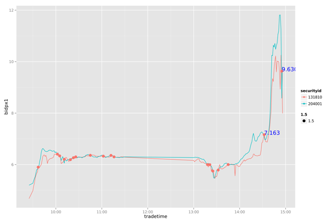
通过对一周数据的比较我们发现,这个简单的策略能我们带来一些收益。虽然不是全局最优的,但比人为的判断会更有依据。
作者介绍:
张丹,R语言中文社区专栏特邀作者,《R的极客理想》系列图书作者,民生银行大数据中心数据分析师,前况客创始人兼CTO。
10年IT编程背景,精通R ,Java, Nodejs 编程,获得10项SUN及IBM技术认证。丰富的互联网应用开发架构经验,金融大数据专家。个人博客 http://fens.me, Alexa全球排名70k。
著有《R的极客理想-工具篇》、《R的极客理想-高级开发篇》,合著《数据实践之美》,新书《R的极客理想-量化投资篇》(即将出版)。

《R的极客理想-工具篇》京东购买快速通道:https://item.jd.com/11524750.html
《R的极客理想-高级开发篇》京东购买快速通道:https://item.jd.com/11731967.html
《数据实践之美》京东购买快速通道:https://item.jd.com/12106224.html
