
作者:李誉辉
四川大学在读研究生
前言
这篇是plot3D包绘图系列之四,前一篇请戳:R_3D图(三),后续还有两篇连载,大家一起加油!做教程狠费精力的,别忘了点赞和转发。谢谢。
4 scatter2D()与scatter3D() 及text2D()与text3D()
point3D()是scatter3D()的特殊形式,参数type = "p"。lines3D()是scatter3D()的特殊形式,参数type = "l"。point2D()是scatter2D()的特殊形式,参数type = "p"。lines2D()是scatter2D()的特殊形式,参数type = "l"。text2D()是另一种不可替代的函数text3D()是另一种不可替代的函数
语法:
scatter3D (x, y, z, ..., colvar = z, phi = 40, theta = 40,

           col = NULL, NAcol = "white", breaks = NULL,

           colkey = NULL, panel.first = NULL,

           clim = NULL, clab = NULL,

           bty = "b", CI = NULL, surf = NULL,

           add = FALSE, plot = TRUE)


text3D (x, y, z, labels, ..., colvar = NULL, phi = 40, theta = 40,

        col = NULL, NAcol = "white",  breaks = NULL,

        colkey = NULL, panel.first = NULL,

        clim = NULL, clab = NULL,

        bty = "b", add = FALSE, plot = TRUE)


points3D (x, y, z, ...)


lines3D (x, y, z, ...)


scatter2D (x, y, ..., colvar = NULL,

         col = NULL, NAcol = "white", breaks = NULL,

         colkey = NULL, clim = NULL, clab = NULL,

         CI = NULL, add = FALSE, plot = TRUE)


lines2D(x, y, ...)


points2D(x, y, ...)


text2D (x, y, labels, ..., colvar = NULL,

         col = NULL, NAcol = "white", breaks = NULL, colkey = NULL,

         clim = NULL, clab = NULL, add = FALSE, plot = TRUE)
参数解释:
x, y, z,表示点的坐标,为数字向量,他们应该等长度,length(x) = length(y) = length(z) 。
colvar,表示指定要着色的变量,默认NULL,如果指定,则长度应等于(x, y, z)。
theta, phi, 表示指定观察方向。与
persp()中一样。col, 表示指定色板,
xxx.col(), 默认NULL,如colvar指定了,则默认红黄蓝的jet.col()颜色。
如果col = NULL,且colvar未指定,则col默认为黑色。NAcol, 表示指定colvar中NA的颜色。
breaks, 表示指定
colvar的断点,为数字向量,长度应该比col参数大1个。
需要增序排列,默认自动增序排列。colkey, 为逻辑值或NULL(默认), 也可以用列表传递
colkey参数。
当colkey = NULL时,若col参数是一个向量,才会自动添加图例,col参数是一个字符串则不添加图例。
设定colkey = list(plot = FALSE)则为图例留下空间,但不显示图例。colkey = FALSE则不绘制图例。CI,为NULL(默认)或列表(包含参数和置信区间数字向量),
如果为列表,则至少应包含x, y, z(z仅仅用于scatter3D()中), 这些参数应该是2列的矩阵,表示左/右间隔。 其它参数应该是:alen = 0.01, lty = par(“lty”), lwd = par(“lwd”), col = NULL,
这几个参数设置箭头的长度,线型,宽度和颜色。 如果col = NULL,则使用colvar指定的颜色。panel.first, 表示指定一种变换函数,常常用于绘制背景网格和三维散点图的平滑处理。 该函数的其中一个参数应该是pmat矩阵变换。见
persp3D()中的例子。clab, 表示指定图例标题内容,当
colkey = NULL或colkey = FALSE时失效。
默认位置于主标题同一高度,降低高度,使用向量指定,第一个元素为空字符串。clim, 表示指定
colvar显示范围,如果colvar参数被指定了,则超出clim范围的colvar将以NA显示。bty, 表示指定box的类型,默认仅仅画背景panels,只有当
persp()中的box = TRUE时才有效。
其它与perspbox()函数中一致,bty = c(“b”, “b2”, “f”, “g”, “bl”, “bl2”, “u”, “n”)其中之一。labels, 表示指定每个散点的的文本标签内容。其长度应等于(x, y, z)。
surf, NULL(默认)或列表传参, 表示增加散点图拟合的曲面,
拟合曲面参数包括: 必要参数(x, y, z指定曲面),
可选参数(colvar, col, NAcol, border, facets, lwd, resfac, clim, ltheta, lphi, shade, lighting, fit)
参数用法与persp()中一样。 默认参数中未指定colvar, 表示默认colvar = z,z的排列应该与scatter3D()中的z一致。add, 表示是否将该绘图对象加入到已存在的绘图对象中,
TRUE相当于增加图层,默认FALSE则新建。plot, 表示是否立即绘图,默认TRUE则立即绘图,FALSE则往下传递绘图参数,直到最后一个图层一起绘制。
…, 表示其它参数,包括公共参数,
persp()中的参数,perspbox()中的一些参数。persp()中的一些参数:xlim, ylim, zlim, xlab, ylab, zlab, main, sub,
r, d, scale, expand, box, axes, nticks, ticktype。
同样xlim,ylim, zlim也只限制坐标轴范围,超出该范围的图形仍然会绘制出来,
使用plotdev()设定图形范围。perspbox()中的一些参数: col.axis, col.panel, lwd.panel, col.grid, lwd.grid。公共参数:alpha透明度,从0(全透明)到1(不透明)。 lty线型,lwd线宽,
shade和lighting没有任何作用。type, 表示指定点或线等绘图几何类型。只有text3D不可取代。
如type = "p"或"b",指定type后,pch,cex,bg等参数就可以使用了。
4.1 scatter2D()与scatter3D()
4.1.1 全矩阵数据源
library(plot3D)


par(bg = "#b3ff99")# par设定背景颜色


M  <- mesh(seq(0, 2*pi, length.out = 100),

            seq(0, pi, length.out = 100))


u  <- M$x ; v  <- M$y

x <- cos(u)*sin(v) # 矩阵Hadamard积,对应元素相乘

y <- sin(u)*sin(v)

z <- cos(v)


#

scatter3D(x, y, z, pch = ".", col = "magenta", # pch点型可以为字符

          cex = 2, colkey = FALSE, # cex设定点的大小

          bty = "u", col.panel = NA) # 手动设定背景, col.panel = NA设定透明背景
4.1.2 type类型
library(plot3D)


# 编一个数据

z <- seq(0, 10, 0.2)

x <- cos(z)

y <- sin(z)*z


# 三维点图与三维文本

scatter3D(x, y, z, phi = 0,   #

          col = ramp.col(col = c("cyan", "magenta"), n = length(z)),   # 指定颜色色板

          pch = 20, cex = 2, ticktype = "detailed",

          bty = "u", col.panel = "#ffffcc", col.grid = "white")


## 添加图层, 添加一个点在三维空间

scatter3D(x = 0, y = 0, z = 0, add = TRUE,

          col = "blue",   # 指定颜色色板

          colkey = FALSE,

          pch = 10, cex = 3, lwd = 3) # pch点型,cex点尺寸,lwd点中线宽


## 添加图层, 添加10个大写字母在三维空间

text3D(x = cos(1:10), y = (sin(1:10)*(1:10) - 1),

       z = 1:10, colkey = FALSE, add = TRUE,

       labels = LETTERS[1:10], col = ramp.col(col = c("blue", "red"), n = 10))
# 三维线图,

scatter3D(x, y, z, phi = 0, type = "l",  # type = "l"连线

          col = ramp.col(col = c("cyan", "magenta"), n = length(z)),   # 指定颜色色板

          ticktype = "detailed", lwd = 4,

          bty = "u", col.panel = "#ffffcc", col.grid = "white")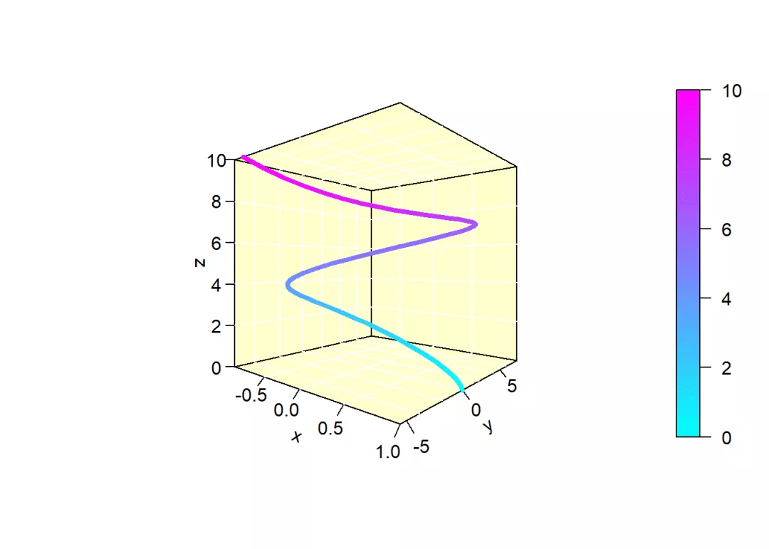
# 三维点图与三维线图

scatter3D(x, y, z, phi = 0, type = "b",# type = "b"表示both,即点连线

          col = ramp.col(col = c("cyan", "magenta"), n = length(z)),   # 指定颜色色板

          bty = "u", col.panel = "#ffffcc", col.grid = "white",

          ticktype = "detailed", pch = 20,

          cex = c(0.5, 1, 1.5))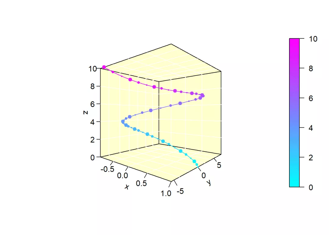
# 竖线条

scatter3D(x, y, z, phi = 0, type = "h",  # type = "h" 点与竖线条

          col = ramp.col(col = c("cyan", "magenta"), n = length(z)),   # 指定颜色色板

          bty = "u", col.panel = "#ffffcc", col.grid = "white",

          ticktype = "detailed")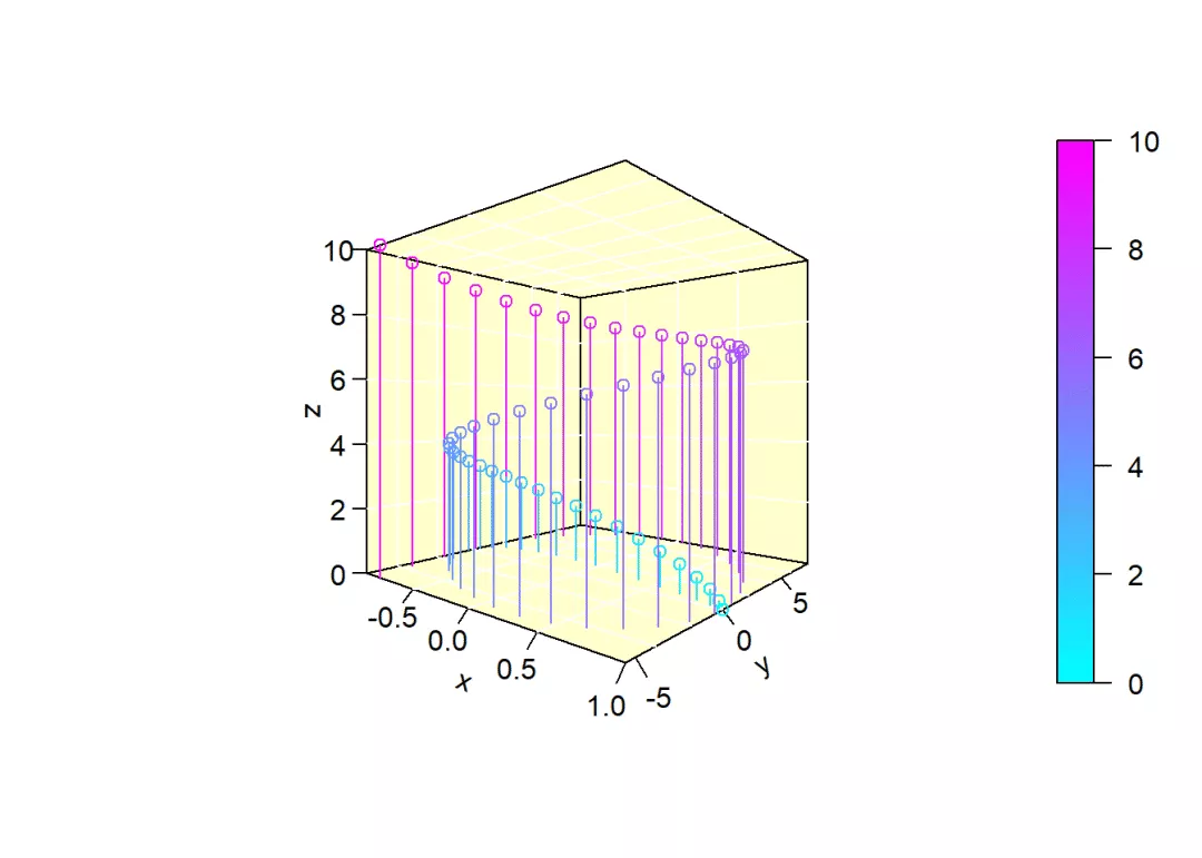
4.1.3 CI置信区间
CI参数为列表,内有1到3个元素,每个元素都是矩阵,其行数和列数length(x)。
表示在各个坐标轴方向上的置信区间,
library(plot3D)


x <- runif(20)  # 20个随机数

y <- runif(20)

z <- runif(20)


## 设定置信区间参数,1个方向的置信区间

CI <- list(z = matrix(nrow = length(x), data = rep(0.05, 2 * length(x))))  # 矩阵行数和列数都是length(x),值均为0.05


# 设定box类型,bty='g'灰色背景,白色grid

scatter3D(x, y, z, theta = 45, phi = 0, bty = "g", CI = CI, col = ramp.col(col = c("cyan",

    "magenta"), n = 100, alpha = 0.8), pch = 19, cex = 2, ticktype = "detailed",

    xlim = c(0, 1), ylim = c(0, 1), zlim = c(0, 1))


# 增加一些散点 点坐标参数

x <- runif(20)

y <- runif(20)

z <- runif(20)


## 设定置信区间参数, 2个方向的置信区间

CI2 <- list(x = matrix(nrow = length(x), data = rep(0.05, 2 * length(x))), z = matrix(nrow = length(x),

    data = rep(0.05, 2 * length(x))))


scatter3D(x, y, z, CI = CI2, add = TRUE, col = "orange", pch = 2)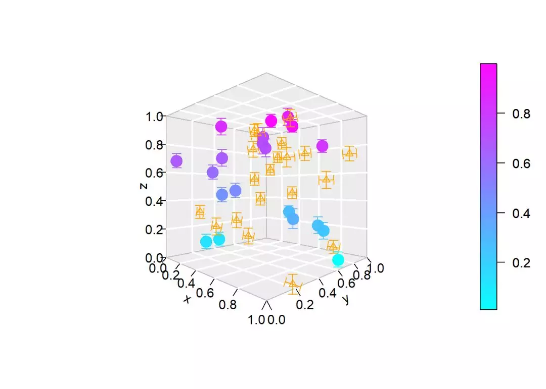
4.1.4 surf添加曲面
surf参数中,可以使用列表传递曲面参数,与persp()中的参数一样。
当传递坐标参数与scatter3D()中无关则相当于添加曲面。
library(plot3D)


M <- mesh(1:nrow(volcano), 1:ncol(volcano))


# 绘制100个点,编坐标参数

N  <- 100

xs <- runif(N) * 87

ys <- runif(N) * 61

zs <- runif(N)*50 + 154


# 绘图,

scatter3D(xs, ys, zs, theta = 45, ticktype = "detailed", pch = 16,

          bty = "f", xlim = c(1, 87), ylim = c(1,61), zlim = c(94, 215), # bty = "f",所有panels透明

          surf = list(x = M$x, y = M$y, z = volcano,

          NAcol = "grey", shade = 0.1))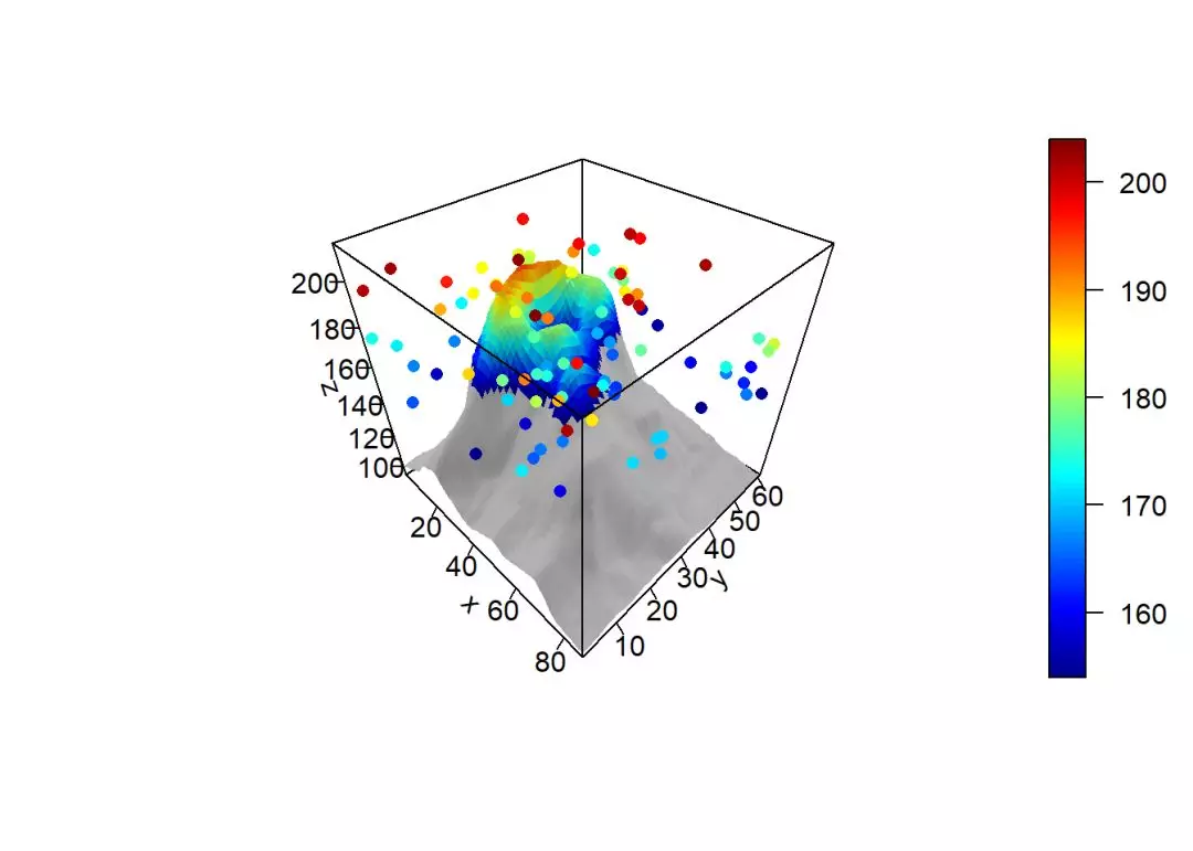
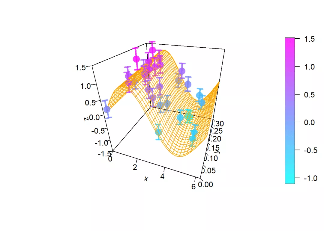
library(plot3D)


# 构建曲面网格坐标

M <- mesh(seq(0, 2*pi, length = 30), (1:30)/100)

z <- with (M, sin(x) + y) #


# 散点图坐标

N <- 30

xs <- runif(N) * 2*pi

ys <- runif(N) * 0.3


zs <- sin(xs) + ys + rnorm(N)*0.3


CI <- list(z = matrix(nrow = length(xs),

                       data = rep(0.3, 2*length(xs))),

           lwd = 3) # CI列表传参还能传递其它参数


# facets = NA,网格面透明,网格线border为黑色

scatter3D(xs, ys, zs, ticktype = "detailed", pch = 16,

          col = ramp.col(col = c("cyan", "magenta"), n = 30, alpha = 0.8),

          xlim = c(0, 2*pi), ylim = c(0, 0.3), zlim = c(-1.5, 1.5),  # 指定坐标轴显示范围

          CI = CI, theta = 20, phi = 30, cex = 2,

          surf = list(x = M$x, y = M$y, z = z, border = "orange", facets = NA)

)
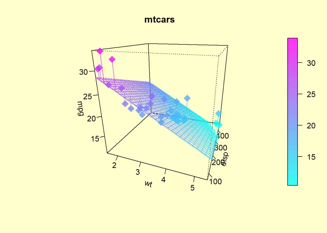
4.1.5 坐标数据来自预测值
在with()内绘图
library(plot3D)


par(bg = "#ffffcc")


with (mtcars, { # with内处理数据并绘图


# 线性回归,多元回归

fit <- lm(mpg ~ wt + disp)


# 构建预测数据

wt.pred <- seq(1.5, 5.5, length.out = 30)

disp.pred <- seq(71, 472, length.out = 30)

xy <- expand.grid(wt = wt.pred, disp = disp.pred) # expand.grid向量构建数据框


## 预测mag值,然后转换成矩阵

mpg.pred <- matrix (nrow = 30, ncol = 30,

                    data = predict(fit, newdata = data.frame(xy),

                                   interval = "prediction")

                    )


# olddata预测

fitpoints <- predict(fit)


scatter3D(z = mpg, x = wt, y = disp, pch = 18, cex = 2,

          theta = 20, phi = 20, ticktype = "detailed",

          col = ramp.col(col = c("cyan", "magenta"), n = 30, alpha = 0.8),

          xlab = "wt", ylab = "disp", zlab = "mpg",  # 修改坐标轴标题

          surf = list(x = wt.pred, y = disp.pred, z = mpg.pred,

                      facets = NA, fit = fitpoints), # fit参数增加预测值与真实值之间的连线

          main = "mtcars", bty = "u", col.panel = NA) # col.panel = NA则panel透明


})
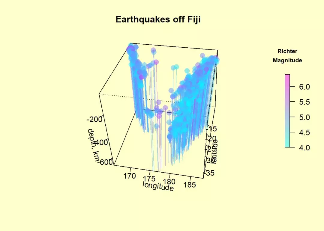
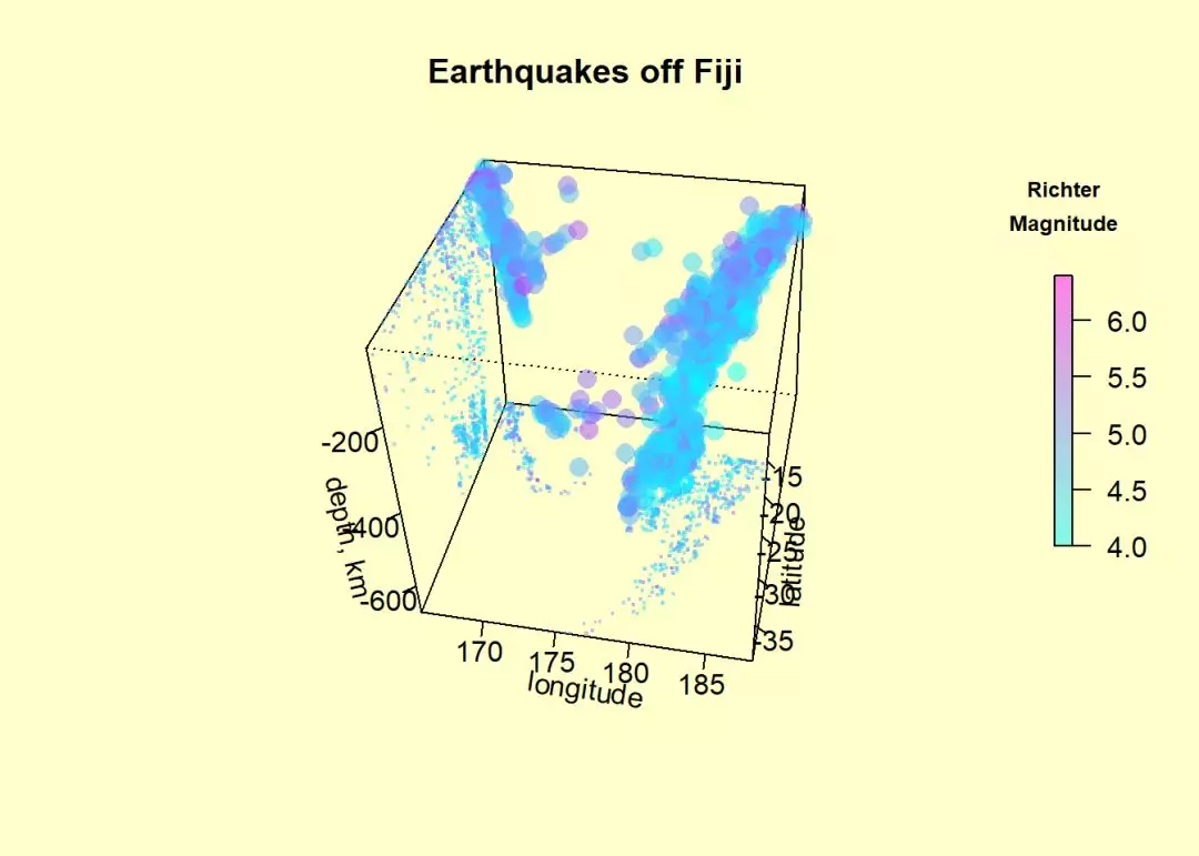
4.1.6 panel.first参数在panel中增加图形
panel.first可以指定绘图对象,也就可以在panels中增加图形。
library(plot3D)

par(bg = "#ffffcc")


# 第一种方法,type = "h"增加垂线条

with(quakes, scatter3D(x = long, y = lat, z = -depth, colvar = mag,

     pch = 16, cex = 1.5, xlab = "longitude", ylab = "latitude",

     col = ramp.col(col = c("cyan", "magenta"), n = length(mag), alpha = 0.5),

     zlab = "depth, km", clab = c("Richter","Magnitude"),

     main = "Earthquakes off Fiji", ticktype = "detailed", bty = "u", col.panel = NA, # 透明面板

     type = "h", theta = 10, d = 2,

     colkey = list(length = 0.5, width = 0.5, cex.clab = 0.75)) # 图例列表传参

)


# 第2中方法,使用trans3D构建转换空间

# 然后使用转换空间绘制二维散点图,再使用panel.first参数将该图add到scatter3D基图中


# 绘制panel.first图

lens <- length(quakes$mag)

panelfirst <- function(pmat) {


  ## 绘制x-y平面的panel

  zmin <- min(-quakes$depth)

  ### trans3D构建转换空间,x,y坐标与第1种方法中一样,z轴仅仅计数,以免重复

  XY <- trans3D(quakes$long, quakes$lat,

                z = rep(zmin, nrow(quakes)), pmat = pmat)

  ### 使用转换空间绘制散点图,必须使用add = TRUE才能将图形以panel.first参数传入基图中

  scatter2D(XY$x, XY$y, colvar = quakes$mag, pch = ".", # colvar着色变量与基图相同

            col = ramp.col(col = c("cyan", "magenta"), n = lens, alpha = 0.5),

            cex = 2, add = TRUE, colkey = FALSE) #


  ## 绘制y-z平面的panel

  xmin <- min(quakes$long) # x轴仅仅计数

  ### trans3D构建转换空间,y,z坐标与第1种方法相同,x轴仅仅计数避免重复

  XY <- trans3D(x = rep(xmin, nrow(quakes)), y = quakes$lat,

                z = -quakes$depth, pmat = pmat)

  ### 使用转换空间绘制散点图,必须使用add = TRUE才能将图形以panel.first参数传入基图中

  scatter2D(XY$x, XY$y, colvar = quakes$mag, pch = ".", # colvar着色变量与基图相同

            col = ramp.col(col = c("cyan", "magenta"), n = lens, alpha = 0.5),

            cex = 2, add = TRUE, colkey = FALSE)

}


# 将panel.first图添加到scatter3D基图中

with(quakes, scatter3D(x = long, y = lat, z = -depth, colvar = mag,

     pch = 16, cex = 1.5, xlab = "longitude", ylab = "latitude",

     col = ramp.col(col = c("cyan", "magenta"), n = length(mag), alpha = 0.5),

     zlab = "depth, km", clab = c("Richter","Magnitude"),

     main = "Earthquakes off Fiji", ticktype = "detailed", bty = "u", col.panel = NA, # 透明面板

     panel.first = panelfirst, theta = 10, d = 2,  # panel.first传递panels绘图对象

     colkey = list(length = 0.5, width = 0.5, cex.clab = 0.75))

)
4.2 text2D()与text3D()
4.2.1 text3D()添加文字
library(plot3D)


par(bg = "#ffffcc")# par设定背景颜色

data("USArrests")


# 绘制散点图与垂线条

scatter3D(USArrests$Murder, USArrests$Assault, USArrests$Rape - 1,

          colvar = USArrests$UrbanPop,

          col = ramp.col(col = c("cyan", "magenta"), n = length(USArrests$UrbanPop), alpha = 0.5),

          colkey = list( length = 0.5, col.clab = "blue", dist = -0.1), # 列表传参,设定图例

          type = "h", pch = ".",bty = "u", col.panel = NA)


# 添加文字

text3D(USArrests$Murder, USArrests$Assault, USArrests$Rape, add = TRUE,

       colvar = USArrests$UrbanPop, theta = 60, phi = 20,

       col = ramp.col(col = c("cyan", "magenta"), n = length(USArrests$UrbanPop), alpha = 0.5),

       xlab = "Murder", ylab = "Assault", zlab = "Rape",

       main = "USA arrests", colkey = FALSE,

       labels = rownames(USArrests), cex = 0.6,

       bty = "u", ticktype = "detailed", d = 2,

       clab = c("Urban","Pop"), adj = 0.5, font = 2, col.panel = NA)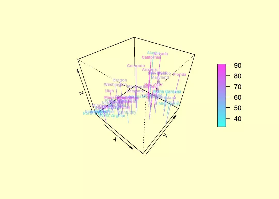
4.2.2 坐标轴刻度文本text
library(plot3D)

data(VADeaths)


hist3D(x = 1:5, y = 1:4, z = VADeaths, expand = 0.5, phi = 20, theta = -72,

    shade = 0.2, itheta = 72, iphi = 60, d = 2, xlab = "", ylab = "", zlab = "",

    main = "VADeaths", col = ramp.col(col = c("cyan", "green"), n = 3, alpha = 0.5)[2],

    border = "magenta", alpha = 0.15, opaque.top = TRUE, bty = "g", space = 0.3,

    ticktype = "detailed", cex.axis = 1e-09)


text3D(x = 1:5, y = rep(0.5, 5), z = rep(3, 5), labels = rownames(VADeaths),

    add = TRUE, adj = 0, col = "magenta", bty = "g")


text3D(x = rep(1, 4), y = 1:4, z = rep(0, 4), labels = colnames(VADeaths), add = TRUE,

    adj = 1, col = "magenta", bty = "g")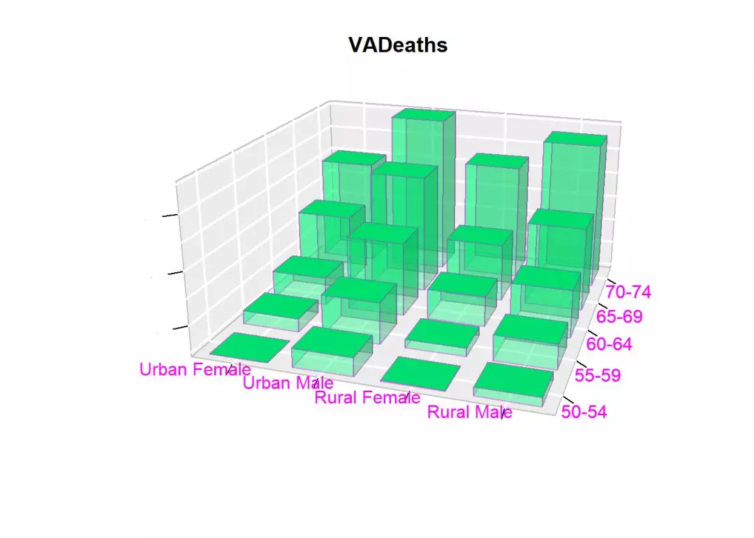
4.3 scatter2D()
4.3.1 type参数
library(plot3D)


par(mfrow = c(2, 2), bg = "#ffffcc") # 多图排版,2*2矩阵排列


x <- seq(0, 2*pi, length.out = 30)


# 默认type为点

scatter2D(x, sin(x), colvar = cos(x), pch = 16,

          col = ramp.col(col = c("cyan", "magenta"), n = 30, alpha = 0.5),

          colkey = list(col.axis = "blue", col.ticks = "green", col.clab = "purple"), # 设定图例参数

          ylab = "sin", clab = "cos", cex = 1.5)


# type = "l"连线

scatter2D(x, sin(x), colvar = cos(x),

          col = ramp.col(col = c("cyan", "magenta"), n = 30, alpha = 0.5),

          colkey = list(col.axis = "blue", col.ticks = "green", col.clab = "purple"), # 设定图例参数

         type = "l", lwd = 4, bty = "g")


# type = "b"点和联系

scatter2D(x, sin(x), colvar = cos(x),

          col = ramp.col(col = c("cyan", "magenta"), n = 30, alpha = 0.5),

          colkey = list(col.axis = "blue", col.ticks = "green", col.clab = "purple"), # 设定图例参数

          type = "b", lwd = 2, bty = "g")


# type = "h"竖线

scatter2D(x, sin(x), colvar = cos(x),

          col = ramp.col(col = c("cyan", "magenta"), n = 30, alpha = 0.5),

          colkey = list(col.axis = "blue", col.ticks = "green", col.clab = "purple"), # 设定图例参数

          type = "h", lwd = 4, alpha = 0.5) # 指定透明的和线宽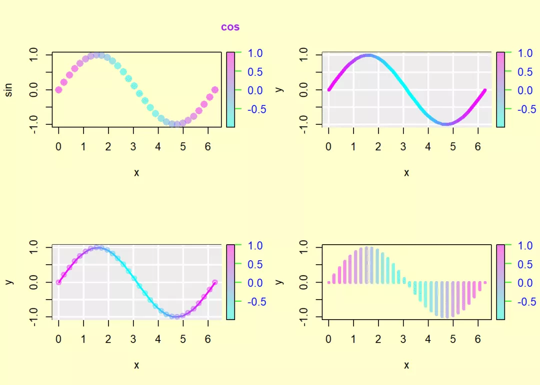
4.3.2 text2D()添加文本
library(plot3D)

data("USArrests")


par(bg = "#ffffcc")


text2D(x = USArrests$Murder, y = USArrests$Assault + 5, colvar = USArrests$Rape,

    col = ramp.col(col = c("cyan", "magenta"), n = length(USArrests$Rape), alpha = 0.5),

    xlab = "Murder", ylab = "Assault", clab = "Rape", main = "USA arrests",

    labels = rownames(USArrests), cex = 0.6, adj = 0.5, font = 2, colkey = list(plot = FALSE))


scatter2D(x = USArrests$Murder, y = USArrests$Assault, colvar = USArrests$Rape,

    col = ramp.col(col = c("cyan", "magenta"), n = length(USArrests$Rape), alpha = 0.8),

    pch = 16, add = TRUE)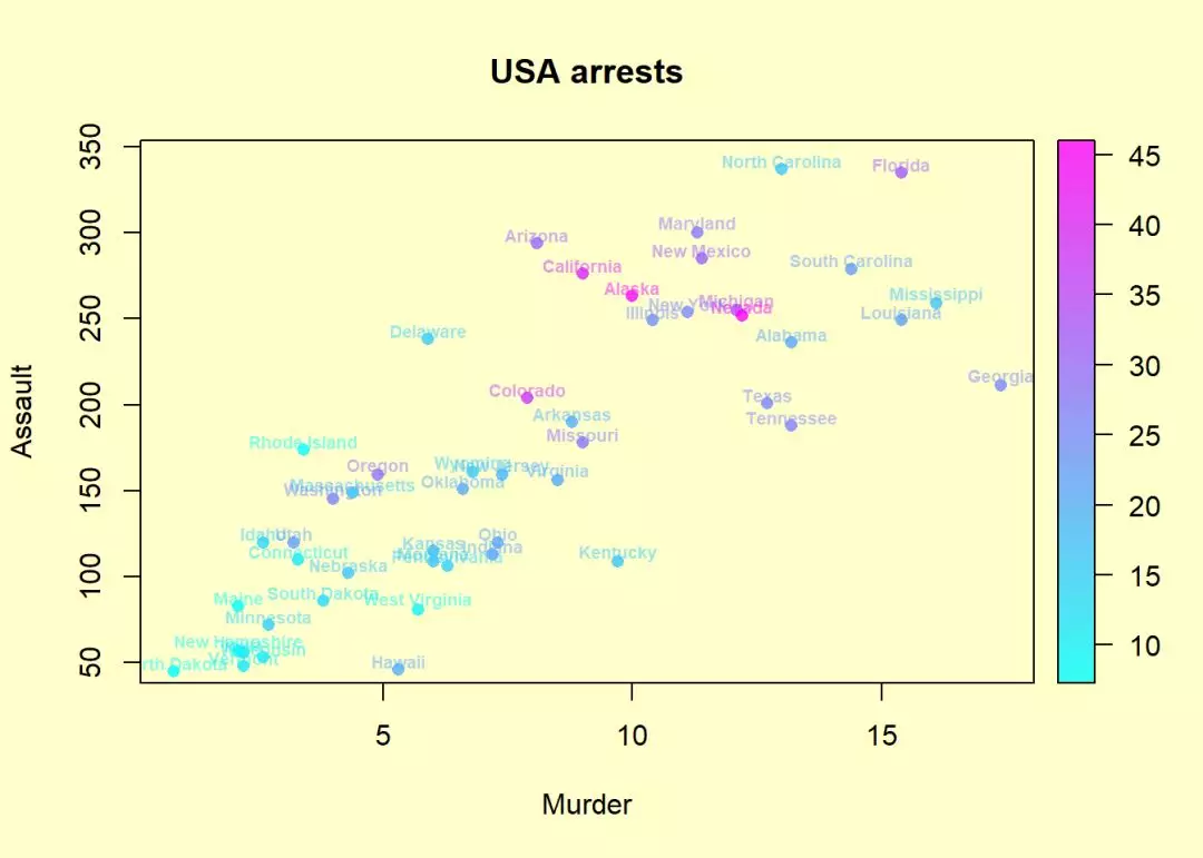
4.3.3 mesh数据源
library(plot3D)


par(mfrow = c(1, 2), bg = "#ffffcc")


x <- seq(-1, 1, by = 0.1)

y <- seq(-2, 2, by = 0.2)


grid <- mesh(x, y)

z <- with(grid, cos(x) * sin(y))


# 第一张图

image2D(x = x, y = y, z = z, col = ramp.col(col = c("cyan", "magenta"), n = length(x),

    alpha = 0.5))

points(grid, col = "blue")  # 使用R自带函数添加图层,设定变量颜色为蓝色


# 第2张图

scatter2D(grid$x, grid$y, colvar = z, pch = 20, cex = 2, col = ramp.col(col = c("cyan",

    "magenta"), n = length(x), alpha = 0.5))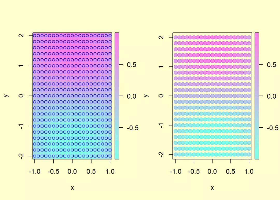
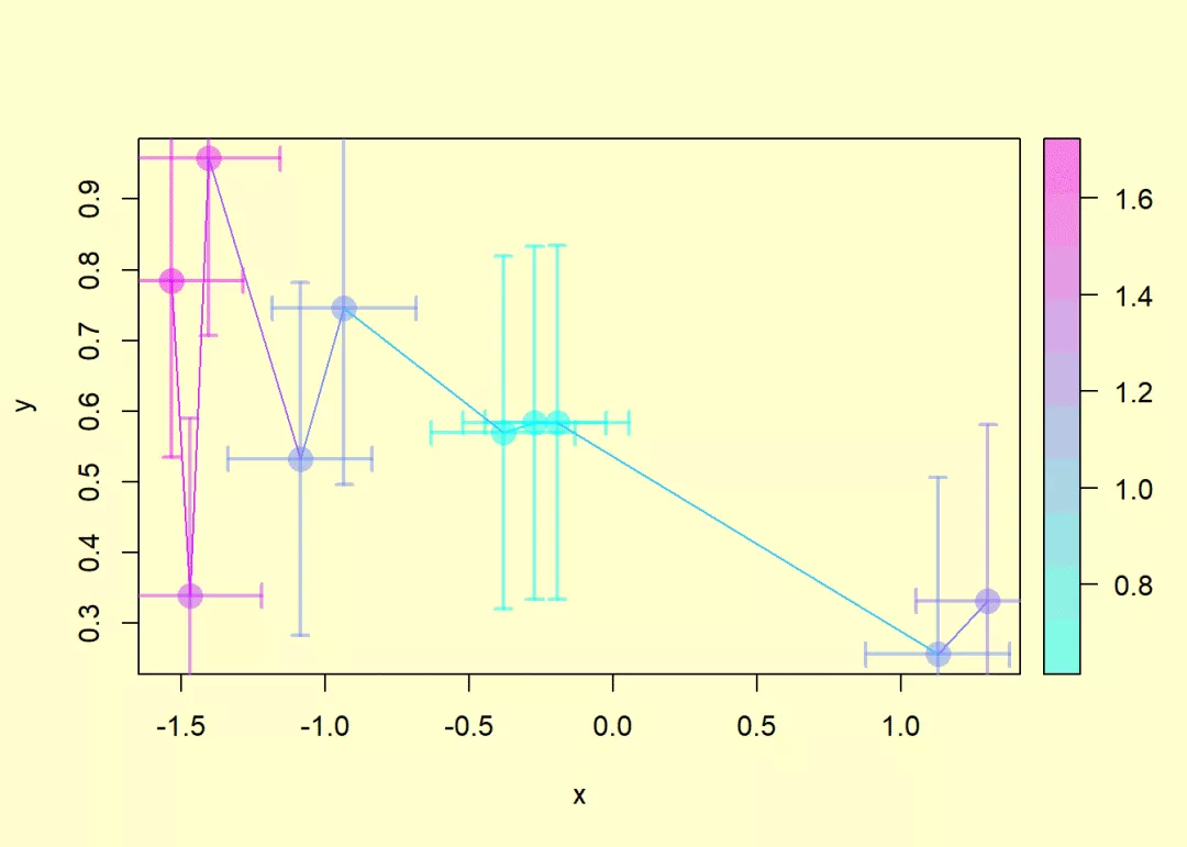
4.3.4 CI置信区间
library(plot3D)
par(bg = "#ffffcc")
x <- sort(rnorm(10))
y <- runif(10)
cv <- sqrt(x^2 + y^2)
# 创建置信区间列表
CI <- list(lwd = 2) # 置信区间线宽
CI$x <- matrix(nrow = length(x), data = c(rep(0.25, 2 * length(x)))) # 给列表增加元素,x方向的置信区间
CI2 <- CI
CI2$y <- matrix(nrow = length(y), data = c(rep(0.25, 2 * length(y)))) # 给列表增加元素,y方向的置信区间
scatter2D(x, y, colvar = cv, col = ramp.col(col = c("cyan", "magenta"), n = length(x),
alpha = 0.5), pch = 16, cex = 2, CI = CI)
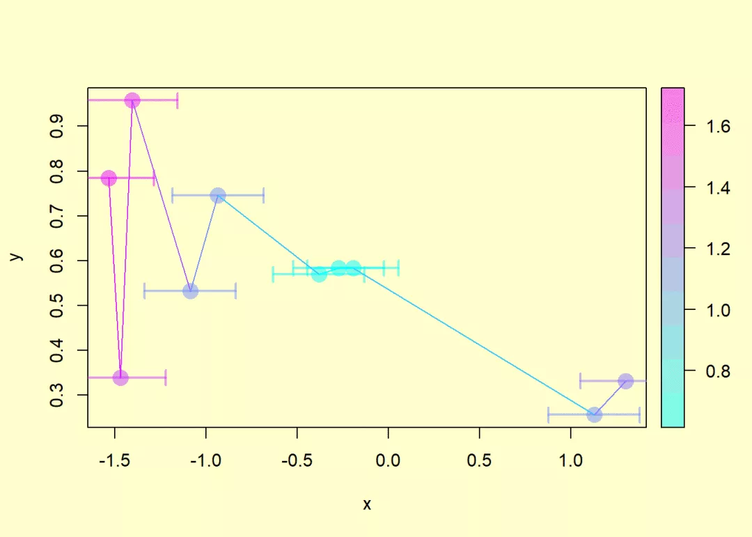
# 更改type = 'b'点连线
scatter2D(x, y, colvar = cv, col = ramp.col(col = c("cyan", "magenta"), n = length(x),
alpha = 0.5), pch = 16, cex = 2, CI = CI, type = "b")
# 增加y方向的置信区间
scatter2D(x, y, colvar = cv, col = ramp.col(col = c("cyan", "magenta"), n = length(x),
alpha = 0.5), pch = 16, cex = 2, CI = CI2, type = "b")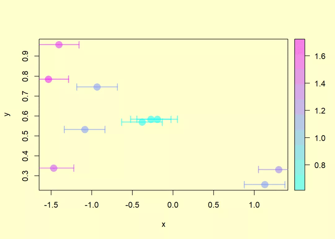
4.3.5 添加绘图对象到地图中
library(plot3D)

data(Oxsat)


# image2D绘制地图

oxlim <- range(Oxsat$val[, , 1], na.rm = TRUE)

image2D(z = Oxsat$val[, , 1], x = Oxsat$lon, y = Oxsat$lat, contour = TRUE,

    xlab = "longitude", ylab = "latitude", main = "Oxygen saturation", clim = oxlim,

    clab = "%")


# 数据点坐标创建

lon <- c(11.2, 6, 0.9, -4, -8.8)

lat <- c(-19.7, -14.45, -9.1, -3.8, -1.5)

O2sat <- c(90, 95, 92, 85, 100)  # 数据点着色变量


# add to image; use same zrange; avoid adding a color key

scatter2D(x = lon, y = lat, colvar = O2sat, clim = oxlim, pch = 16, add = TRUE,

    cex = 2, colkey = FALSE)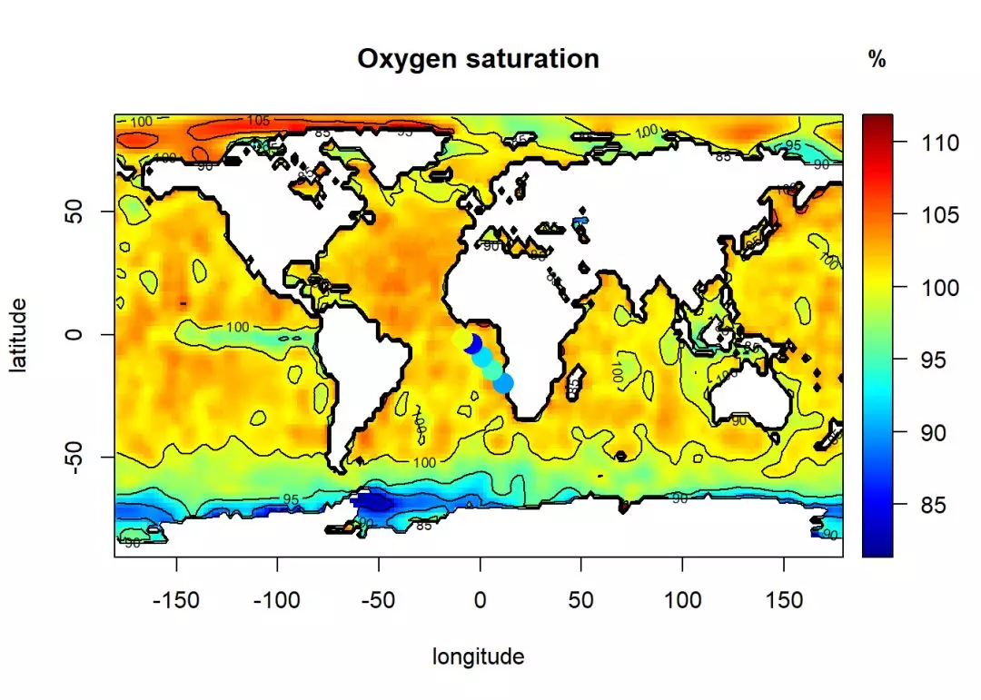
4.4 line2D()
与scatter2D()中type = "l"结果一样
library(plot3D)

data("sunspot.month")


par(bg = "#ffffcc")


# 筛选数据

sunspot <- data.frame(year = time(sunspot.month),

                      anom = sunspot.month - mean(sunspot.month))


ff <- 100

sunspot$ma <- filter(sunspot$anom, rep(1/ff, ff), sides = 2)


# type = "h"绘制垂线条

lines2D(sunspot$year, sunspot$anom, colvar = sunspot$anom > 0,

        col = ramp.col(col = c("pink", "lightblue"), n = 2, alpha = 0.1), # 正数一种颜色,负数一种颜色

        main = "sunspot anomaly", type = "h",

        colkey = FALSE, las = 1, xlab = "year", ylab = "")


# tyep = "l"绘制连线,注意着色变量不一样

lines2D(sunspot$year, sunspot$ma, add = TRUE,

col = ramp.col(col = c("green", "magenta"), n = length(sunspot$ma), alpha = 0.9)) 

····
往期精彩:
····


公众号后台回复关键字即可学习
回复 爬虫 爬虫三大案例实战
回复 Python 1小时破冰入门回复 数据挖掘 R语言入门及数据挖掘
回复 人工智能 三个月入门人工智能
回复 数据分析师 数据分析师成长之路
回复 机器学习 机器学习的商业应用
回复 数据科学 数据科学实战
回复 常用算法 常用数据挖掘算法