
作者:yangyang541 R语言中文社区专栏作者
1 简介
近几年开始着手汇市预测与投资模式,分别使用了ARIMA、ETS、GARCH等等统计模型。在比较了多模型后,GJR-GARCH预测最为精准,然而在默认模型下并没有将ARIMA(p,d,q)值最优化。
原文:哥哥姐姐,请问IGARCH模型的参数估计怎么编程实现啊.,此文章添加解释与一些参考文献,并且测试3年移动数据以确定新GARCH模型是否更为精准。
suppressPackageStartupMessages(require('BBmisc'))

## 读取程序包

pkg <- c('lubridate', 'plyr', 'dplyr', 'magrittr', 'stringr', 'rugarch', 'forecast', 'quantmod', 'microbenchmark', 'knitr', 'kableExtra', 'formattable')

suppressAll(lib(pkg))

rm(pkg)无意中发现,分享下rugarch中的GARCH模式最优化…
2 数据
首先读取Binary.com Interview Q1 (Extention)的汇市数据。
cr_code <- c('AUDUSD=X', 'EURUSD=X', 'GBPUSD=X', 'CHF=X', 'CAD=X',

             'CNY=X', 'JPY=X')

#'@ names(cr_code) <- c('AUDUSD', 'EURUSD', 'GBPUSD', 'USDCHF', 'USDCAD',

#'@                     'USDCNY', 'USDJPY')

names(cr_code) <- c('USDAUD', 'USDEUR', 'USDGBP', 'USDCHF', 'USDCAD', 'USDCNY', 'USDJPY')

price_type <- c('Op', 'Hi', 'Lo', 'Cl')

## 读取雅虎数据。

mbase <- sapply(names(cr_code), function(x) readRDS(paste0('./data/', x, '.rds')) %>% na.omit)
数据简介报告。
sapply(mbase, summary) %>%

  kable %>%

  kable_styling(bootstrap_options = c('striped', 'hover', 'condensed', 'responsive')) %>%

  scroll_box(width = '100%', height = '400px')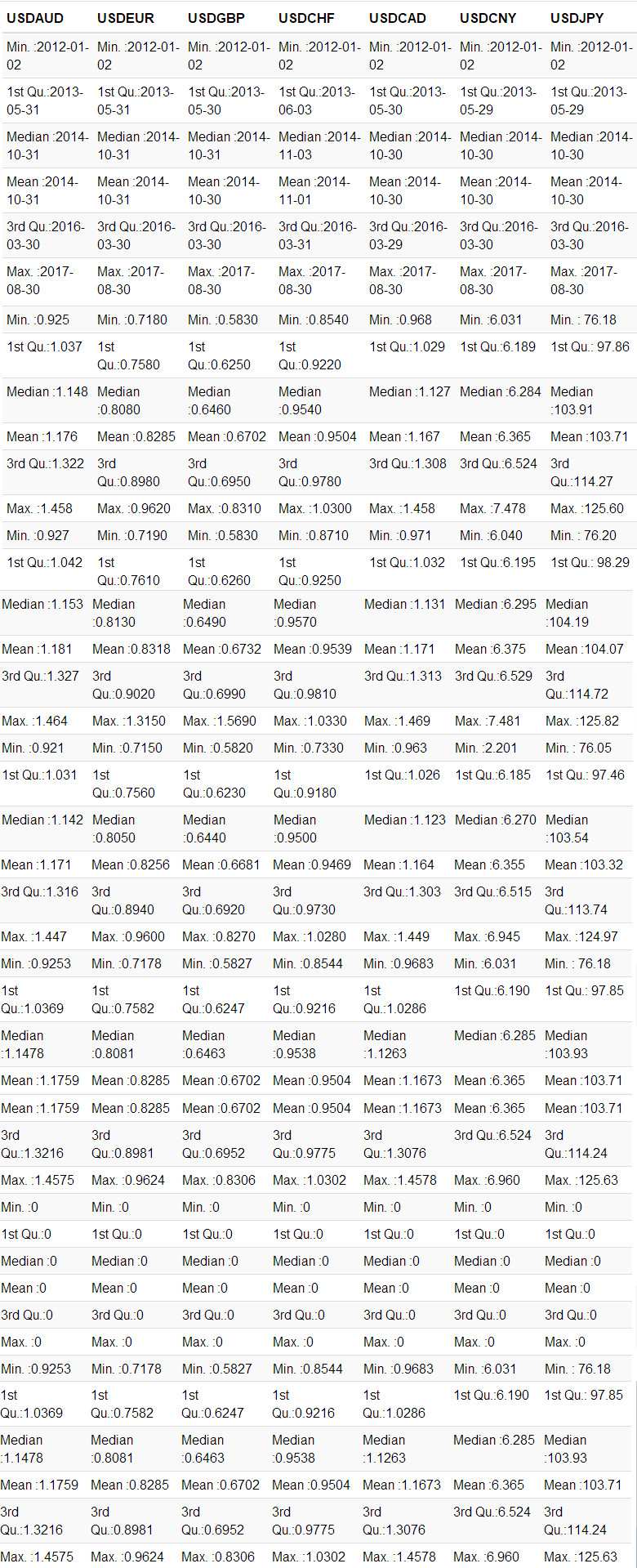
桌面2.1:数据简介。
3 统计建模
3.1 基础模型
fGarch : Various submodels arise from this model, and are passed to the ugarchspec “variance.model” list via the submodel option,
- The simple GARCH model of Bollerslev (1986) when λ=δ=2λ=δ=2 and η1j=η2j=0η1j=η2j=0(submodel = ‘GARCH’).
- The Absolute Value GARCH (AVGARCH) model of Taylor (1986) and Schwert (1990) when λ=δ=1λ=δ=1 and |η1j|≤1|η1j|≤1 (submodel = ‘AVGARCH’).
- The GJR GARCH (GJRGARCH) model of Glosten et al. (1993) when λ=δ=2λ=δ=2 and η2j=0η2j=0 (submodel = ‘GJRGARCH’).
- The Threshold GARCH (TGARCH) model of Zakoian (1994) when λ=δ=1,η2j=0λ=δ=1,η2j=0 and |η1j|≤1|η1j|≤1 (submodel = ‘TGARCH’).
- The Nonlinear ARCH model of Higgins et al. (1992) when δ=λδ=λ and η1j=η2j=0η1j=η2j=0(submodel = ‘NGARCH’).
- The Nonlinear Asymmetric GARCH model of Engle and Ng (1993) when δ=λ=2δ=λ=2 and η1j=0η1j=0 (submodel = ‘NAGARCH’).
- The Asymmetric Power ARCH model of Ding et al. (1993) when δ=λ,η2j=0δ=λ,η2j=0 and |η1j|≤1|η1j|≤1 (submodel = ‘APARCH’).
- The Exponential GARCH model of Nelson (1991) when δ=1,λ=0δ=1,λ=0 and η2j=0η2j=0 (not implemented as a submodel of fGARCH).
- The Full fGARCH model of Hentschel (1995) when δ=λδ=λ (submodel = ‘ALLGARCH’).
The choice of distribution is entered via the ‘distribution.model’ option of the ugarchspec method. The package also implements a set of functions to work with the parameters of these distributions. These are:
ddist(distribution = "norm", y, mu = 0, sigma = 1, lambda = -0.5, skew = 1, shape = 5). The density (d*) function.pdist(distribution = "norm", q, mu = 0, sigma = 1, lambda = -0.5, skew = 1, shape = 5). The distribution (p*) function.qdist(distribution = "norm", p, mu = 0, sigma = 1, lambda = -0.5, skew = 1, shape = 5). The quantile (q*) function.rdist(distribution = "norm", n, mu = 0, sigma = 1, lambda = -0.5, skew = 1, shape = 5). The sampling (q*) function.fitdist(distribution = "norm", x, control = list()). A function for fitting data using any of the included distributions.dskewness(distribution = "norm", skew = 1, shape = 5, lambda = -0.5). The distribution skewness (analytical where possible else by quadrature integration).dkurtosis(distribution = "norm", skew = 1, shape = 5, lambda = -0.5). The distribution excess kurtosis (analytical where it exists else by quadrature integration).
The family of APARCH models includes the ARCH and GARCH models, and five other ARCH extensions as special cases:
- ARCH Model of Engle when δ=2δ=2, γi=0γi=0, and βj=0βj=0.
- GARCH Model of Bollerslev when δ=2δ=2, and γi=0γi=0.
- TS-GARCH Model of Taylor and Schwert when δ=1δ=1, and γi=0γi=0.
- GJR-GARCH Model of Glosten, Jagannathan, and Runkle when δ=2δ=2.
- T-ARCH Model of Zakoian when δ=1δ=1.
- N-ARCH Model of Higgens and Bera when γi=0γi=0, and βj=0βj=0.
- Log-ARCH Model of Geweke and Pentula when δ→0δ→0.
原文:Parameter Estimation of ARMA Models with GARCH/APARCH Errors - An R and SPlus Software Implementation文献中的2. Mean and Variance Equation。
有关多种GARCH模式比较,请参考参考文献中的链接3… 包括比较:
- auto.arima
- exponential smoothing models (ETS)
- GARCH (包括GARCH、eGARCH、iGARCH、fGARCH、gjrGARCH等模式)
- exponential weighted models
σ2t=ω+∑i=1ρ(αi+γiIt−i)ε2t−i+∑j=1qβjσ2t−j ⋯ Equation 3.1.1σt2=ω+∑i=1ρ(αi+γiIt−i)εt−i2+∑j=1qβjσt−j2 ⋯ Equation 3.1.1
在之前的文章已经分别比较多种统计模式,得知GJR-GARCH模型的预测结果最为精准,以下稍微介绍下平滑移动加权模型。
3.2 ARMA 模型
ARMA Mean Equation: The
ARMA(p,q)process of autoregressive orderpand moving average orderqcan be described as
xt=μ+∑i=1mαixt−i+∑j=1nβjεt−j+εt=μ+α(B)xt+β(B)εt⋯ Equation 3.2.1xt=μ+∑i=1mαixt−i+∑j=1nβjεt−j+εt=μ+α(B)xt+β(B)εt⋯ Equation 3.2.1
以上函数乃滑动加权指数,请参阅以下链接以了解更多详情:
- Computer Lab Sessions 2&3
- 時間序列分析 - 總體經濟與財務金融之應用 - 定態時間序列II ARMA模型
- Introduction to the rugarch package
- Parameter Estimation of ARMA Models with GARCH/APARCH Errors - An R and SPlus Software Implementation
- How to choose the order of a GARCH model?
3.3 GJR-GARCH:ARMA(p,q)值最优化(旧程序)
使用极大似然法计算最优arma order中的p值与q值,将原本默认值最优化,让模型马尔可夫化,每日的p与q值最将会使用最佳值… 不包括d值。
armaSearch <- suppressWarnings(function(data, .method = 'CSS-ML') {

    ## I set .method = 'CSS-ML' as default method since the AIC value we got is

    ##  smaller than using method 'ML' while using method 'CSS' facing error.

    ##

    ## https://stats.stackexchange.com/questions/209730/fitting-methods-in-arima

    ## According to the documentation, this is how each method fits the model:

    ##  - CSS minimises the sum of squared residuals.

    ##  - ML maximises the log-likelihood function of the ARIMA model.

    ##  - CSS-ML mixes both methods: first, CSS is run, the starting parameters

    ##    for the optimization algorithm are set to zeros or to the values given

    ##    in the optional argument init; then, ML is applied passing the CSS

    ##    parameter estimates as starting parameter values for the optimization algorithm.


    .methods = c('CSS-ML', 'ML', 'CSS')


    if(!.method %in% .methods)

      stop(paste('Kindly choose .method among ',

                 paste0(.methods, collapse = ', '), '!'))


    armacoef <- data.frame()

    for (p in 0:5){

      for (q in 0:5) {

        #data.arma = arima(diff(data), order = c(p, 0, q))

        #'@ data.arma = arima(data, order = c(p, 1, q), method = .method)

        if(.method == 'CSS-ML') {

          data.arma = tryCatch({

            arma = arima(data, order = c(p, 1, q), method = 'CSS-ML')

            mth = 'CSS-ML'

            list(arma, mth)

          }, error = function(e) tryCatch({

            arma = arima(data, order = c(p, 1, q), method = 'ML')

            mth = 'ML'

            list(arma = arma, mth = mth)

          }, error = function(e) {

            arma = arima(data, order = c(p, 1, q), method = 'CSS')

            mth = 'CSS'

            list(arma = arma, mth = mth)

          }))


        } else if(.method == 'ML') {

          data.arma = tryCatch({

            arma = arima(data, order = c(p, 1, q), method = 'ML')

            mth = 'ML'

            list(arma = arma, mth = mth)

          }, error = function(e) tryCatch({

            arma = arima(data, order = c(p, 1, q), method = 'CSS-ML')

            mth = 'CSS-ML'

            list(arma = arma, mth = mth)

          }, error = function(e) {

            arma = arima(data, order = c(p, 1, q), method = 'CSS')

            mth = 'CSS'

            list(arma = arma, mth = mth)

          }))


        } else if(.method == 'CSS') {

          data.arma = tryCatch({

            arma = arima(data, order = c(p, 1, q), method = 'CSS')

            mth = 'CSS'

            list(arma = arma, mth = mth)

          }, error = function(e) tryCatch({

            arma = arima(data, order = c(p, 1, q), method = 'CSS-ML')

            mth = 'CSS-ML'

            list(arma = arma, mth = mth)

          }, error = function(e) {

            arma = arima(data, order = c(p, 1, q), method = 'ML')

            mth = 'ML'

            list(arma = arma, mth = mth)

          }))


        } else {

          stop(paste('Kindly choose .method among ', paste0(.methods, collapse = ', '), '!'))

        }

        names(data.arma) <- c('arma', 'mth')


        #cat('p =', p, ', q =', q, 'AIC =', data.arma$arma$aic, '\n')

        armacoef <- rbind(armacoef,c(p, q, data.arma$arma$aic))

      }

    }


    ## ARMA Modeling寻找AIC值最小的p,q

    colnames(armacoef) <- c('p', 'q', 'AIC')

    pos <- which(armacoef$AIC == min(armacoef$AIC))

    cat(paste0('method = \'', data.arma$mth, '\', the min AIC = ', armacoef$AIC[pos],

               ', p = ', armacoef$p[pos], ', q = ', armacoef$q[pos], '\n'))

    return(armacoef)

  })
然后把以上的函数嵌入以下GARCH模型,将原本固定参数的ARMA值浮动化。
calC <- function(mbase, currency = 'JPY=X', ahead = 1, price = 'Cl') {


  # Using "memoise" to automatically cache the results

  source('function/filterFX.R')

  source('function/armaSearch.R')

  mbase = suppressWarnings(filterFX(mbase, currency = currency, price = price))


  armaOrder = suppressWarnings(armaSearch(mbase))

  armaOrder %<>% dplyr::filter(AIC == min(AIC)) %>% .[c('p', 'q')] %>% unlist


  spec = ugarchspec(

    variance.model = list(

      model = 'gjrGARCH', garchOrder = c(1, 1),

      submodel = NULL, external.regressors = NULL,

      variance.targeting = FALSE),

    mean.model = list(

      armaOrder = armaOrder,

      include.mean = TRUE, archm = FALSE,

      archpow = 1, arfima = FALSE,

      ## https://stats.stackexchange.com/questions/73351/how-does-one-specify-arima-p-d-q-in-ugarchspec-for-ugarchfit-in-rugarch?answertab=votes#tab-top

      ## https://d.cosx.org/d/2689-2689/9

      external.regressors = NULL,

      archex = FALSE),

    distribution.model = 'snorm')

  fit = ugarchfit(spec, mbase, solver = 'hybrid')

  fc = ugarchforecast(fit, n.ahead = ahead)

  res = tail(attributes(fc)$forecast$seriesFor, 1)

  colnames(res) = names(mbase)

  latestPrice = tail(mbase, 1)

  #rownames(res) <- as.character(forDate)

  latestPrice <- xts(latestPrice)

  #res <- as.xts(res)


  tmp = list(latestPrice = latestPrice, forecastPrice = res,

             AIC = infocriteria(fit))

  return(tmp)

}
3.4 Fi-GJR-GARCH:ARFIMA(p,d,q)值最优化(新程序)
The fractionally integrated GARCH model (‘fiGARCH’) : Contrary to the case of the ARFIMA model, the degree of persistence in the FIGARCH model operates in the oppposite direction, so that as the fractional differencing parameter d gets closer to one, the memory of the FIGARCH process increases, a direct result of the parameter acting on the squared errors rather than the conditional variance. When
d = 0the FIGARCH collapses to the vanilla GARCH model and whend = 1to the integrated GARCH model…Motivated by the developments in long memory processes, and in particular the ARFIMA type models (see section 2.1), Baillie et al. (1996) proposed the fractionally integrated generalized autoregressive conditional heteroscedasticity, or FIGARCH, model to capture long memory (in essence hyperbolic memory). Unlike the standard GARCH where shocks decay at an exponential rate, or the integrated GARCH model where shocks persist forever, in the FIGARCH model shocks decay at a slower hyperbolic rate. Consider the standard GARCH equation:
σ2t=ω+α(L)ε2t+β(L)σ2⋯ Equation 3.1.2σt2=ω+α(L)εt2+β(L)σ2⋯ Equation 3.1.2
原文:Introduction to the rugarch package文献中的2.2.10 The fractionally integrated GARCH model (‘fiGARCH’)
然后计算最优arma order… 也包括d值。
opt_arma <- function(mbase){

  #ARMA Modeling minimum AIC value of `p,d,q`

  fit <- auto.arima(mbase)

  arimaorder(fit)

}再来就设置Garch模型中的arfima参数,将原本固定的d值浮动化。
calc_fx <- function(mbase, currency = 'JPY=X', ahead = 1, price = 'Cl') {


  ## Using "memoise" to automatically cache the results

  ## http://rpubs.com/englianhu/arma-order-for-garch

  source('function/filterFX.R')

  #'@ source('function/armaSearch.R') #old optimal arma p,q value searching, but no d value.

  source('function/opt_arma.R') #rename the function best.ARMA()


  mbase = suppressWarnings(filterFX(mbase, currency = currency, price = price))

  armaOrder = opt_arma(mbase)


  ## Set arma order for `p, d, q` for GARCH model.

  #'@ https://stats.stackexchange.com/questions/73351/how-does-one-specify-arima-p-d-q-in-ugarchspec-for-ugarchfit-in-rugarch

  spec = ugarchspec(

    variance.model = list(

      model = 'gjrGARCH', garchOrder = c(1, 1),

      submodel = NULL, external.regressors = NULL,

      variance.targeting = FALSE),

    mean.model = list(

      armaOrder = armaOrder[c(1, 3)], #set arma order for `p` and `q`.

      include.mean = TRUE, archm = FALSE,

      archpow = 1, arfima = TRUE, #set arima = TRUE

      external.regressors = NULL,

      archex = FALSE),

    fixed.pars = list(arfima = armaOrder[2]), #set fixed.pars for `d` value

    distribution.model = 'snorm')


  fit = ugarchfit(spec, mbase, solver = 'hybrid')


  fc = ugarchforecast(fit, n.ahead = ahead)

  #res = xts::last(attributes(fc)$forecast$seriesFor)

  res = tail(attributes(fc)$forecast$seriesFor, 1)

  colnames(res) = names(mbase)

  latestPrice = tail(mbase, 1)

  #rownames(res) <- as.character(forDate)

  latestPrice <- xts(latestPrice)

  #res <- as.xts(res)


  tmp = list(latestPrice = latestPrice, forecastPrice = res,

             AIC = infocriteria(fit))

  return(tmp)

  }
4 模式比较
4.1 运行时间
首先比较运行时间,哪个比较高效。
## 测试运行时间。

#'@ microbenchmark(fit <- calc_fx(mbase[[names(cr_code)[sp]]], currency = cr_code[sp]))

#'@ microbenchmark(fit2 <- calC(mbase[[names(cr_code)[sp]]], currency = cr_code[sp]))

## 随机抽样货币数据,测试运行时间。

sp <- sample(1:7, 1)

system.time(fit1 <- calc_fx(mbase[[names(cr_code)[sp]]], currency = cr_code[sp]))
## user system elapsed
## 8.240 0.024 8.382system.time(fit2 <- calC(mbase[[names(cr_code)[sp]]], currency = cr_code[sp]))## method = 'CSS-ML', the min AIC = -11085.3927792844, p = 5, q = 2## user system elapsed
## 12.82 0.00 13.61由于使用microbenchmark非常耗时,而且双方实力悬殊,故此僕使用system.time()比较运行速度,结果还是新程序calc_fx()比旧程序calC()迅速。
4.2 数据误差率
以下僕运行数据测试后事先储存,然后直接读取。首先过滤timeID时间参数,然后才模拟预测汇价。
#'@ ldply(mbase, function(x) range(index(x)))

#     .id         V1         V2

#1 USDAUD 2012-01-02 2017-08-30

#2 USDEUR 2012-01-02 2017-08-30

#3 USDGBP 2012-01-02 2017-08-30

#4 USDCHF 2012-01-02 2017-08-30

#5 USDCAD 2012-01-02 2017-08-30

#6 USDCNY 2012-01-02 2017-08-30

#7 USDJPY 2012-01-02 2017-08-30

timeID <- llply(mbase, function(x) as.character(index(x))) %>%

  unlist %>% unique %>% as.Date %>% sort

timeID <- c(timeID, xts::last(timeID) + days(1)) #the last date + 1 in order to predict the next day of last date to make whole dataset completed.

timeID0 <- ymd('2013-01-01')

timeID <- timeID[timeID >= timeID0]

## ---------------- 6个R进程并行运作 --------------------

start <- seq(1, length(timeID), ceiling(length(timeID)/6))

#[1]    1  204  407  610  813 1016

stop <- c((start - 1)[-1], length(timeID))

#[1]  203  406  609  812 1015 1217

cat(paste0('\ntimeID <- timeID[', paste0(start, ':', stop), ']'), '\n')
##
## timeID <- timeID[1:203]
## timeID <- timeID[204:406]
## timeID <- timeID[407:609]
## timeID <- timeID[610:812]
## timeID <- timeID[813:1015]
## timeID <- timeID[1016:1217]#timeID <- timeID[1:203]
#timeID <- timeID[204:406]
#timeID <- timeID[407:609]
#timeID <- timeID[610:812]
#timeID <- timeID[813:1015]
#timeID <- timeID[1016:1217]
## Some currency data doesn't open market in speficic date.
#Error:
#data/fx/USDCNY/pred1.2015-04-15.rds saved! #only USDJPY need to review
#data/fx/USDGBP/pred1.2015-12-07.rds saved! #only USDCHF need to review
#data/fx/USDCAD/pred1.2016-08-30.rds saved! #only USDCNY need to review
#data/fx/USDAUD/pred1.2016-11-30.rds saved! #only USDEUR need to review
#data/fx/USDCNY/pred1.2017-01-12.rds saved! #only USDJPY need to review
#data/fx/USDEUR/pred1.2017-02-09.rds saved! #only USDGBP need to review
#timeID <- timeID[timeID > ymd('2017-03-08')]
#data/fx/USDCAD/pred2.2015-06-09.rds saved! #only USDCNY need to review
#data/fx/USDCAD/pred2.2015-06-16.rds saved! #only USDCNY need to review
#data/fx/USDCAD/pred2.2015-06-17.rds saved! #only USDCNY need to review模拟calC()函数预测汇价数据。
## ------------- 模拟calC()预测汇价 ----------------------

pred1 <- list()

for (dt in timeID) {


  for (i in seq(cr_code)) {


    smp <- mbase[[names(cr_code)[i]]]

    dtr <- xts::last(index(smp[index(smp) < dt]), 1) #tail(..., 1)

    smp <- smp[paste0(dtr %m-% years(1), '/', dtr)]


    pred1[[i]] <- ldply(price_type, function(y) {

      df = calC(smp, currency = cr_code[i], price = y)

      df = data.frame(Date = index(df[[1]][1]),

                      Type = paste0(names(df[[1]]), '.', y),

                      df[[1]], df[[2]], t(df[[3]]))

      names(df)[4] %<>% str_replace_all('1', 'T+1')

      df

    })


    if (!dir.exists(paste0('data/fx/', names(pred1[[i]])[3])))

      dir.create(paste0('data/fx/', names(pred1[[i]])[3]))


    saveRDS(pred1[[i]], paste0(

      'data/fx/', names(pred1[[i]])[3], '/pred1.',

      unique(pred1[[i]]$Date), '.rds'))


    cat(paste0(

      'data/fx/', names(pred1[[i]])[3], '/pred1.',

      unique(pred1[[i]]$Date), '.rds saved!\n'))


    }; rm(i)

}查询模拟测试进度的函数task_progress()如下。
task_progress <- function(scs = 60, .pattern = '^pred1', .loops = TRUE) {

  ## ------------- 定时查询进度 ----------------------

  ## 每分钟自动查询与更新以上模拟calC()预测汇价进度(储存文件量)。


  if (.loops == TRUE) {

    while(1) {

      cat('Current Tokyo Time :', as.character(now('Asia/Tokyo')), '\n\n')


      z <- ldply(mbase, function(dtm) {

        y = index(dtm)

        y = y[y >= timeID0]


        cr = as.character(unique(substr(names(dtm), 1, 6)))

        x = list.files(paste0('./data/fx/', cr), pattern = .pattern) %>%

          str_extract_all('[0-9]{4}-[0-9]{2}-[0-9]{2}') %>%

          unlist %>% as.Date %>% sort

        x = x[x >= y[1] & x <= xts::last(y)]


        data.frame(.id = cr, x = length(x), n = length(y)) %>%

        mutate(progress = percent(x/n))

      })# %>% tbl_df


      print(z)


      prg = sum(z$x)/sum(z$n)

      cat('\n================', as.character(percent(prg)), '================\n\n')


      if (prg == 1) break #倘若进度达到100%就停止更新。


      Sys.sleep(scs) #以上ldply()耗时3~5秒,而休息时间60秒。

    }

  } else {


    cat('Current Tokyo Time :', as.character(now('Asia/Tokyo')), '\n\n')


    z <- ldply(mbase, function(dtm) {

      y = index(dtm)

      y = y[y >= timeID0]


      cr = as.character(unique(substr(names(dtm), 1, 6)))

      x = list.files(paste0('./data/fx/', cr), pattern = .pattern) %>%

          str_extract_all('[0-9]{4}-[0-9]{2}-[0-9]{2}') %>%

          unlist %>% as.Date %>% sort

      x = x[x >= y[1] & x <= xts::last(y)]


      data.frame(.id = cr, x = length(x), n = length(y)) %>%

        mutate(progress = percent(x/n))

      })# %>% tbl_df


    print(z)


    prg = sum(z$x)/sum(z$n)

    cat('\n================', as.character(percent(prg)), '================\n\n')

    }

}模拟calc_fx()函数预测汇价数据。
## ------------- 模拟calc_fx()预测汇价 ----------------------

pred2 <- list()

for (dt in timeID) {


  for (i in seq(cr_code)) {


    smp <- mbase[[names(cr_code)[i]]]

    dtr <- xts::last(index(smp[index(smp) < dt]), 1) #tail(..., 1)

    smp <- smp[paste0(dtr %m-% years(1), '/', dtr)]


    pred2[[i]] <- ldply(price_type, function(y) {

      df = calc_fx(smp, currency = cr_code[i], price = y)

      df = data.frame(Date = index(df[[1]][1]),

                      Type = paste0(names(df[[1]]), '.', y),

                      df[[1]], df[[2]], t(df[[3]]))

      names(df)[4] %<>% str_replace_all('1', 'T+1')

      df

    })


    if (!dir.exists(paste0('data/fx/', names(pred2[[i]])[3])))

      dir.create(paste0('data/fx/', names(pred2[[i]])[3]))


    saveRDS(pred2[[i]], paste0(

      'data/fx/', names(pred2[[i]])[3], '/pred2.',

      unique(pred2[[i]]$Date), '.rds'))


    cat(paste0(

      'data/fx/', names(pred2[[i]])[3], '/pred2.',

      unique(pred2[[i]]$Date), '.rds saved!\n'))


    }; rm(i)

  }
模拟完毕后,再来就查看数据结果。
## calC()模拟数据误差率

task_progress(.pattern = '^pred1', .loops = FALSE)
## Current Tokyo Time : 2018-09-07 04:27:06
##
## .id x n progress
## 1 USDAUD 1214 1215 99.92%
## 2 USDEUR 1214 1215 99.92%
## 3 USDGBP 1215 1216 99.92%
## 4 USDCHF 1214 1215 99.92%
## 5 USDCAD 1214 1214 100.00%
## 6 USDCNY 1214 1215 99.92%
## 7 USDJPY 1213 1215 99.84%
##
## ================ 99.92% ================## calc_fx()模拟数据误差率
task_progress(.pattern = '^pred2', .loops = FALSE)## Current Tokyo Time : 2018-09-07 04:27:06
##
## .id x n progress
## 1 USDAUD 1215 1215 100.00%
## 2 USDEUR 1215 1215 100.00%
## 3 USDGBP 1216 1216 100.00%
## 4 USDCHF 1215 1215 100.00%
## 5 USDCAD 1214 1214 100.00%
## 6 USDCNY 1212 1215 99.75%
## 7 USDJPY 1215 1215 100.00%
##
## ================ 99.96% ================以上结果显示,模拟后的数据的误差率非常渺小1。以下筛选pred1与pred2同样日期的有效数据。
##数据1

fx1 <- llply(names(cr_code), function(x) {

    fls <- list.files(paste0('data/fx/', x), pattern = '^pred1')

    dfm <- ldply(fls, function(y) {

        readRDS(paste0('data/fx/', x, '/', y))

    }) %>% data.frame(Cat = 'pred1', .) %>% tbl_df

    names(dfm)[4:5] <- c('Price', 'Price.T1')

    dfm

 })

names(fx1) <- names(cr_code)

##数据2

fx2 <- llply(names(cr_code), function(x) {

    fls <- list.files(paste0('data/fx/', x), pattern = '^pred2')

    dfm <- ldply(fls, function(y) {

        readRDS(paste0('data/fx/', x, '/', y))

    }) %>% data.frame(Cat = 'pred2', .) %>% tbl_df

    names(dfm)[4:5] <- c('Price', 'Price.T1')

    dfm

 })

names(fx2) <- names(cr_code)

#合并,并且整理数据。

fx1 %<>% ldply %>% tbl_df

fx2 %<>% ldply %>% tbl_df

fx <- suppressAll(bind_rows(fx1, fx2) %>% arrange(Date) %>%

  mutate(.id = factor(.id), Cat = factor(Cat)) %>%

  ddply(.(Cat, Type), function(x) {

    x %>% mutate(Price.T1 = lag(Price.T1, 1))

  }) %>% tbl_df %>%

    dplyr::filter(Date >= ymd('2013-01-01') & Date <= ymd('2017-08-30')))

rm(fx1, fx2)
## filter all predictive error where sd >= 20%.
notID <- fx %>% mutate(diff = abs(Price.T1/Price), se = ifelse(diff <= 0.8 | diff >= 1.25, 1, 0)) %>% dplyr::filter(se == 1)
ntimeID <- notID %>% .$Date %>% unique
notID %>%
kable(caption = 'Error data') %>%
kable_styling(bootstrap_options = c('striped', 'hover', 'condensed', 'responsive')) %>%
scroll_box(width = '100%', height = '400px')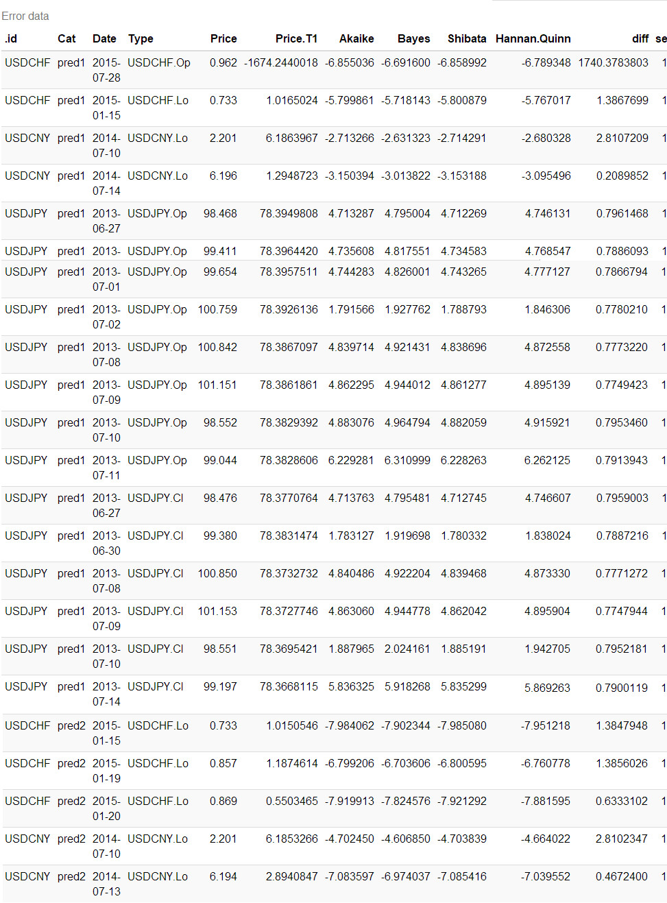
僕尝试运行好几次,USDCHF都是获得同样的结果。然后将默认的snorm分布更换为norm就没有出现错误。至于USDCNY原始数据有误就不是统计模型的问题了。
fx %<>% dplyr::filter(!Date %in% ntimeID)4.3 精准度
现在就比较下双方的MSE值与AIC值。
acc <- ddply(fx, .(Cat, Type), summarise,

             mse = mean((Price.T1 - Price)^2),

             n = length(Price),

             Akaike.mse = (-2*mse)/n+2*4/n,

             Akaike = mean(Akaike),

             Bayes = mean(Bayes),

             Shibata = mean(Shibata),

             Hannan.Quinn = mean(Hannan.Quinn)) %>%

  tbl_df %>% mutate(mse = round(mse, 6)) %>%

  arrange(Type)

acc %>%

  kable(caption = 'Group Table Summary') %>%

  kable_styling(bootstrap_options = c('striped', 'hover', 'condensed', 'responsive')) %>%

  group_rows('USD/AUD Open', 1, 2, label_row_css = 'background-color: #e68a00; color: #fff;') %>%

  group_rows('USD/AUD High', 3, 4, label_row_css = 'background-color: #e68a00; color: #fff;') %>%

  group_rows('USD/AUD Low', 5, 6, label_row_css = 'background-color: #e68a00; color: #fff;') %>%

  group_rows('USD/AUD Close', 7, 8, label_row_css = 'background-color: #e68a00; color: #fff;') %>%

  group_rows('USD/EUR Open', 9, 10, label_row_css = 'background-color: #6666ff; color: #fff;') %>%

  group_rows('USD/EUR High', 11, 12, label_row_css = 'background-color: #6666ff; color: #fff;') %>%

  group_rows('USD/EUR Low', 13, 14, label_row_css = 'background-color:#6666ff; color: #fff;') %>%

  group_rows('USD/EUR Close', 15, 16, label_row_css = 'background-color: #6666ff; color: #fff;') %>%

  group_rows('USD/GBP Open', 17, 18, label_row_css = 'background-color: #339966; color: #fff;') %>%

  group_rows('USD/GBP High', 19, 20, label_row_css = 'background-color: #339966; color: #fff;') %>%

  group_rows('USD/GBP Low', 21, 22, label_row_css = 'background-color: #339966; color: #fff;') %>%

  group_rows('USD/GBP Close', 23, 24, label_row_css = 'background-color: #339966; color: #fff;') %>%

  group_rows('USD/CHF Open', 25, 26, label_row_css = 'background-color: #808000; color: #fff;') %>%

  group_rows('USD/CHF High', 27, 28, label_row_css = 'background-color: #808000; color: #fff;') %>%

  group_rows('USD/CHF Low', 29, 30, label_row_css = 'background-color: #808000; color: #fff;') %>%

  group_rows('USD/CHF Close', 31, 32, label_row_css = 'background-color: #808000; color: #fff;') %>%

  group_rows('USD/CAD Open', 33, 34, label_row_css = 'background-color: #666; color: #fff;') %>%

  group_rows('USD/CAD High', 35, 36, label_row_css = 'background-color: #666; color: #fff;') %>%

  group_rows('USD/CAD Low', 37, 38, label_row_css = 'background-color: #666; color: #fff;') %>%

  group_rows('USD/CAD Close', 39, 40, label_row_css = 'background-color: #666; color: #fff;') %>%

  group_rows('USD/CNY Open', 41, 42, label_row_css = 'background-color: #e60000; color: #fff;') %>%

  group_rows('USD/CNY High', 43, 44, label_row_css = 'background-color: #e60000; color: #fff;') %>%

  group_rows('USD/CNY Low', 45, 46, label_row_css = 'background-color: #e60000; color: #fff;') %>%

  group_rows('USD/CNY Close', 47, 48, label_row_css = 'background-color: #e60000; color: #fff;') %>%

  group_rows('USD/JPY Open', 49, 50, label_row_css = 'background-color: #ff3377; color: #fff;') %>%

  group_rows('USD/JPY High', 51, 52, label_row_css = 'background-color: #ff3377; color: #fff;') %>%

  group_rows('USD/JPY Low', 53, 54, label_row_css = 'background-color: #ff3377; color: #fff;') %>%

  group_rows('USD/JPY Close', 55, 56, label_row_css = 'background-color: #ff3377; color: #fff;') %>%

  scroll_box(width = '100%', height = '400px')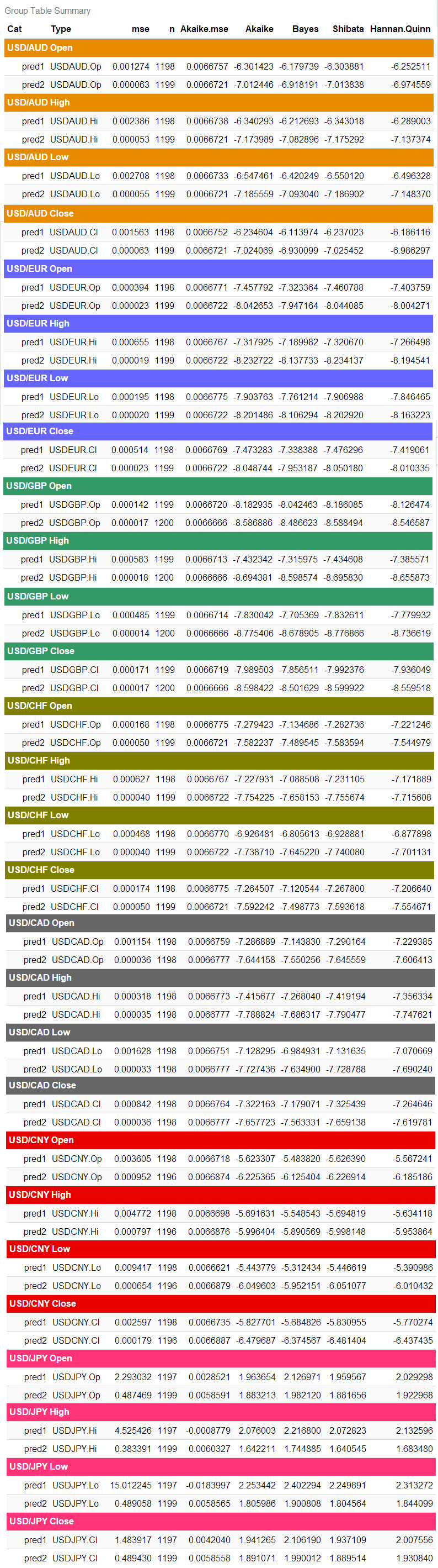
acc <- ddply(fx, .(Cat, .id), summarise,

             mse = mean((Price.T1 - Price)^2),

             n = length(Price),

             Akaike.mse = (-2*mse)/n+2*4/n,

             Akaike = mean(Akaike),

             Bayes = mean(Bayes),

             Shibata = mean(Shibata),

             Hannan.Quinn = mean(Hannan.Quinn)) %>%

  tbl_df %>% mutate(mse = round(mse, 6)) %>%

  arrange(.id)

acc %>%

  kable(caption = 'Group Table Summary') %>%

  kable_styling(bootstrap_options = c('striped', 'hover', 'condensed', 'responsive')) %>%

  group_rows('USD/AUD', 1, 2, label_row_css = 'background-color: #003399; color: #fff;') %>%

  group_rows('USD/CAD', 3, 4, label_row_css = 'background-color: #003399; color: #fff;') %>%

  group_rows('USD/CHF', 5, 6, label_row_css = 'background-color: #003399; color: #fff;') %>%

  group_rows('USD/CNY', 7, 8, label_row_css = 'background-color: #003399; color: #fff;') %>%

  group_rows('USD/EUR', 9, 10, label_row_css = 'background-color: #003399; color: #fff;') %>%

  group_rows('USD/GBP', 11, 12, label_row_css = 'background-color: #003399; color: #fff;') %>%

  group_rows('USD/JPY', 13, 14, label_row_css = 'background-color: #003399; color: #fff;') %>%

  scroll_box(width = '100%', height = '400px')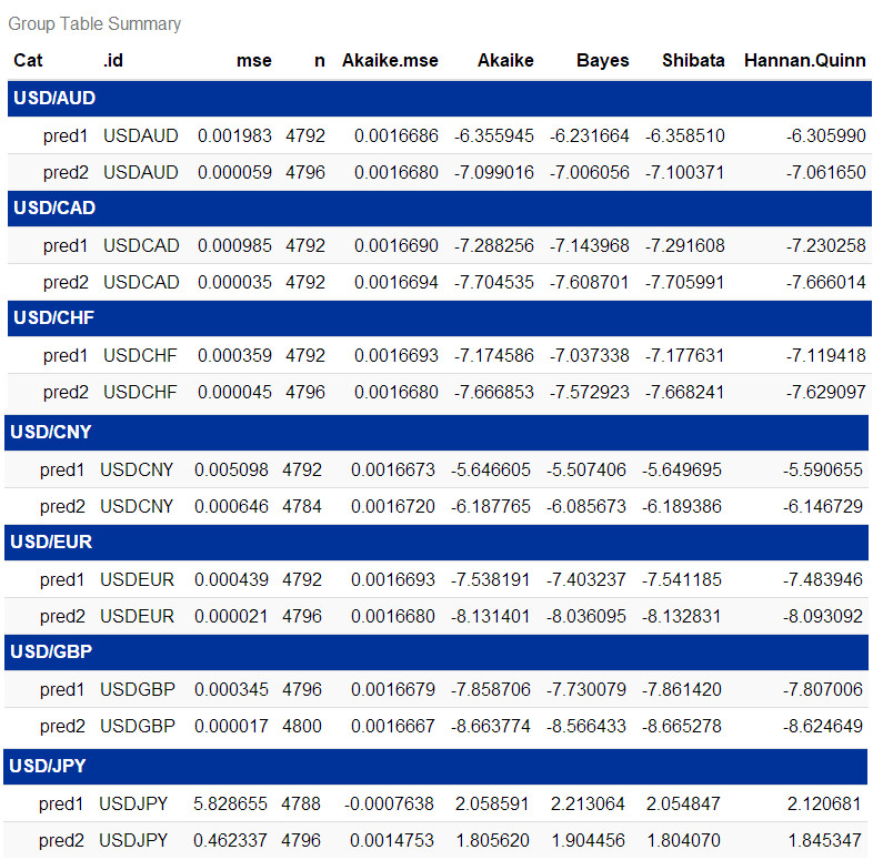
acc <- ddply(fx, .(Cat), summarise,

             mse = mean((Price.T1 - Price)^2),

             n = length(Price),

             Akaike.mse = (-2*mse)/n+2*4/n,

             Akaike = mean(Akaike),

             Bayes = mean(Bayes),

             Shibata = mean(Shibata),

             Hannan.Quinn = mean(Hannan.Quinn)) %>%

  tbl_df %>% mutate(mse = round(mse, 6))

acc %>%

  kable(caption = 'Group Table Summary') %>%

  kable_styling(bootstrap_options = c('striped', 'hover', 'condensed', 'responsive'))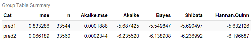
5 结论
结果新的Fi-gjrGARCH函数pred2胜出,比旧的gjrGARCH的pred1更优秀,证明p值、d值与q值仨都可以优化。目前正在编写着Q1App2自动交易应用。“商场如战场”,除了模式最优化以外,程序运作上分秒必争… microbenchmark测试效率,之前编写了个DataCollection应用采集实时数据以方便之后的高频率交易自动化建模2。欲知更多详情,请参阅Real Time FXCM。
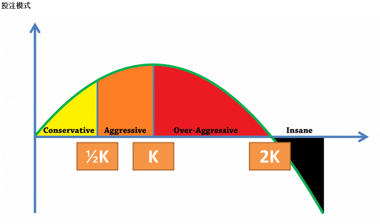
除此之外,由于k=12k=12凯里模式开始时期的增长率比k=1高,故此k值可设置为0.5 ≤ k ≤ 1。Application of Kelly Criterion model in Sportsbook Investment科研也将着手於凯里模式中的k值浮动化。
6 附录
6.1 文件与系统资讯
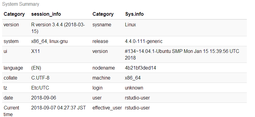
以下乃此文献资讯:
- 文件建立日期:2018-08-07
- 文件最新更新日期:2018-09-07
- R version 3.4.4 (2018-03-15)
- R语言版本:3.4.4
- rmarkdown 程序包版本:1.10.8
- 文件版本:1.0.1
- 作者简历:®γσ, Eng Lian Hu
- GitHub:源代码
- 其它系统资讯:
6.2 参考文献
- How does one specify arima (p,d,q) in ugarchspec for ugarchfit in rugarch?
- How to read p,d and q of auto.arima()?
- binary.com : Job Application - Quantitative Analyst
Powered by - Copyright® Intellectual Property Rights of Scibrokes®個人の経営企業
一些数据模拟时,出现不知名错误。↩
不过数据量多就会当机,得继续提升才行。