深度学习笔记3：手动搭建深度神经网络（DNN）

发表: 2018-07-12 浏览: 1597

R语言 Python

作者简介：
鲁伟：一个数据科学践行者的学习日记。数据挖掘与机器学习，R与Python，理论与实践并行。
个人公众号：数据科学家养成记（微信ID：louwill12）

在笔记 1 和 2 里笔者使用 numpy 手动搭建了感知机单元与一个单隐层的神经网络，理解了神经网络的基本架构和传播原理，掌握了如何从零开始手写一个神经网络。但以上仅是神经网络和深度学习的基础内容，深度学习的一大特征就在于隐藏层之深。因而，我们就这前面的思路，继续利用 numpy 工具，手动搭建一个 DNN 深度神经网络。

再次回顾一下之前我们在搭建神经网络时所秉持的思路和步骤：

定义网络结构
初始化模型参数
循环计算：前向传播/计算当前损失/反向传播/权值更新

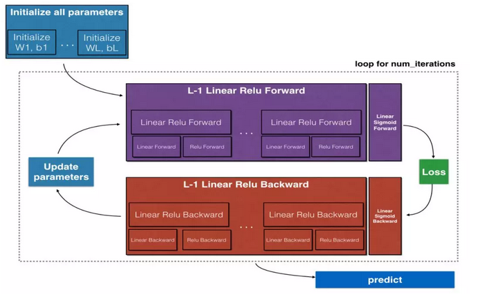
神经网络的计算流程

初始化模型参数

对于一个包含L层的隐藏层深度神经网络，我们在初始化其模型参数的时候需要更灵活一点。我们可以将网络结构作为参数传入初始化函数里面：

def initialize_parameters_deep(layer_dims):

    np.random.seed(3)

    parameters = {}    
    # number of layers in the network

    L = len(layer_dims)            



    for l in range(1, L):

        parameters['W' + str(l)] = np.random.randn(layer_dims[l], layer_dims[l-1])*0.01

        parameters['b' + str(l)] = np.zeros((layer_dims[l], 1))  
      
    assert(parameters['W' + str(l)].shape == (layer_dims[l], layer_dims[l-1]))        
    assert(parameters['b' + str(l)].shape == (layer_dims[l], 1))
    return parameters

以上代码中，我们将参数 layer_dims 定义为一个包含网络各层维数的 list ，使用随机数和归零操作来初始化权重 W 和偏置 b 。

比如说我们指定一个输入层大小为 5 ，隐藏层大小为 4 ，输出层大小为 3 的神经网络，调用上述参数初始化函数效果如下：

parameters = initialize_parameters_deep([5,4,3])

print("W1 = " + str(parameters["W1"]))

print("b1 = " + str(parameters["b1"]))

print("W2 = " + str(parameters["W2"]))

print("b2 = " + str(parameters["b2"]))

W1 = [[ 0.01788628  0.0043651   0.00096497 -0.01863493 -0.00277388]  [-0.00354759 -0.00082741 -0.00627001 -0.00043818 -0.00477218]  [-0.01313865  0.00884622  0.00881318  0.01709573  0.00050034]  [-0.00404677 -0.0054536  -0.01546477  0.00982367 -0.01101068]] 
b1 = [[0.]  [0.]  [0.]  [0.]] 
W2 = [[-0.01185047 -0.0020565   0.01486148  0.00236716]  [-0.01023785 -0.00712993  0.00625245 -0.00160513]  [-0.00768836 -0.00230031  0.00745056  0.01976111]] 
b2 = [[0.]  [0.]  [0.]]

前向传播

前向传播的基本过程就是执行加权线性计算和对线性计算的结果进行激活函数处理的过程。除了此前常用的 sigmoid 激活函数，这里我们引入另一种激活函数 ReLU ，那么这个 ReLU 又是个什么样的激活函数呢？

ReLU

ReLU 全称为线性修正单元，其函数形式表示为 y = max(0, x).
从统计学本质上讲，ReLU 其实是一种断线回归函数，其主要功能在于能在计算反向传播时缓解梯度消失的情形。相对书面一点就是，ReLU 具有稀疏激活性的优点。关于ReLU的更多细节，这里暂且按下不表，我们继续定义深度神经网络的前向计算函数：

def linear_activation_forward(A_prev, W, b, activation):

    if activation == "sigmoid":

        Z, linear_cache = linear_forward(A_prev, W, b)

        A, activation_cache = sigmoid(Z)    
    elif activation == "relu":

        Z, linear_cache = linear_forward(A_prev, W, b)

        A, activation_cache = relu(Z)   
     
    assert (A.shape == (W.shape[0], A_prev.shape[1]))

    cache = (linear_cache, activation_cache)    
    return A, cache

在上述代码中，参数 A_prev 为前一步执行前向计算的结果，中间使用了一个激活函数判断，对两种不同激活函数下的结果分别进行了讨论。

对于一个包含L层采用 ReLU 作为激活函数，最后一层采用 sigmoid 激活函数，前向计算流程如下图所示。

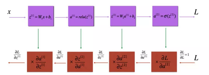
定义L层神经网络的前向计算函数为：

def L_model_forward(X, parameters):

    caches = []

    A = X    
    # number of layers in the neural network

    L = len(parameters) // 2                 



    # Implement [LINEAR -> RELU]*(L-1)

    for l in range(1, L):

        A_prev = A 

        A, cache = linear_activation_forward(A_prev, parameters["W"+str(l)], parameters["b"+str(l)], "relu")

        caches.append(cache)    
    # Implement LINEAR -> SIGMOID

    AL, cache = linear_activation_forward(A, parameters["W"+str(L)], parameters["b"+str(L)], "sigmoid")

    caches.append(cache)    
    
    assert(AL.shape == (1,X.shape[1]))    
    return AL, caches

计算当前损失

有了前向传播的计算结果之后，就可以根据结果值计算当前的损失大小。定义计算损失函数为：

def compute_cost(AL, Y):

    m = Y.shape[1]    
    # Compute loss from aL and y.

    cost = -np.sum(np.multiply(Y,np.log(AL))+np.multiply(1-Y,np.log(1-AL)))/m



    cost = np.squeeze(cost)  
       

    assert(cost.shape == ())    
    return cost

执行反向传播

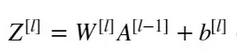
执行反向传播的关键在于正确的写出关于权重 W 和偏置b 的链式求导公式，对于第 l层而言，其线性计算可表示为：

响应的第l层的W 和 b 的梯度计算如下：

由上分析我们可定义线性反向传播函数和线性激活反向传播函数如下：

def linear_backward(dZ, cache):

    A_prev, W, b = cache

    m = A_prev.shape[1]



    dW = np.dot(dZ, A_prev.T)/m

    db = np.sum(dZ, axis=1, keepdims=True)/m

    dA_prev = np.dot(W.T, dZ)    

    assert (dA_prev.shape == A_prev.shape)    
    assert (dW.shape == W.shape)    
    assert (db.shape == b.shape)    
    
    return dA_prev, dW, db

def linear_activation_backward(dA, cache, activation):

    linear_cache, activation_cache = cache    
    if activation == "relu":

        dZ = relu_backward(dA, activation_cache)

        dA_prev, dW, db = linear_backward(dZ, linear_cache)    
    elif activation == "sigmoid":

        dZ = sigmoid_backward(dA, activation_cache)

        dA_prev, dW, db = linear_backward(dZ, linear_cache)    
    return dA_prev, dW, db

根据以上两个反向传播函数，我们可继续定义L层网络的反向传播函数：

def L_model_backward(AL, Y, caches):

    grads = {}

    L = len(caches) 
    # the number of layers

    m = AL.shape[1]

    Y = Y.reshape(AL.shape) 
    # after this line, Y is the same shape as AL



    # Initializing the backpropagation

    dAL = - (np.divide(Y, AL) - np.divide(1 - Y, 1 - AL))    
    # Lth layer (SIGMOID -> LINEAR) gradients

    current_cache = caches[L-1]

    grads["dA" + str(L)], grads["dW" + str(L)], grads["db" + str(L)] = linear_activation_backward(dAL, current_cache, "sigmoid")    
    for l in reversed(range(L - 1)):

        current_cache = caches[l]

        dA_prev_temp, dW_temp, db_temp = linear_activation_backward(grads["dA" + str(l + 2)], current_cache, "relu")

        grads["dA" + str(l + 1)] = dA_prev_temp

        grads["dW" + str(l + 1)] = dW_temp

        grads["db" + str(l + 1)] = db_temp    
    return grads

反向传播涉及大量的复合函数求导计算，所以这一块需要一定的微积分基础。这也是为什么数学是深度学习人工智能的基石所在。

权值更新

反向传播计算完成后，即可根据反向计算结果对权值参数进行更新，定义参数更新函数如下：

def update_parameters(parameters, grads, learning_rate):
    # number of layers in the neural network

    L = len(parameters) // 2 

    # Update rule for each parameter. Use a for loop.

    for l in range(L):

        parameters["W" + str(l+1)] = parameters["W"+str(l+1)] - learning_rate*grads["dW"+str(l+1)]

        parameters["b" + str(l+1)] = parameters["b"+str(l+1)] - learning_rate*grads["db"+str(l+1)]    

    return parameters

封装搭建过程

到此一个包含$$层隐藏层的深度神经网络就搭建好了。当然了，跟前面保持统一，也需要 pythonic的精神，我们继续对全过程的各个函数进行统一封装，定义一个封装函数：

def L_layer_model(X, Y, layers_dims, learning_rate = 0.0075, num_iterations = 3000, print_cost=False):

    np.random.seed(1)

    costs = []    



    # Parameters initialization.

    parameters = initialize_parameters_deep(layers_dims)    
    # Loop (gradient descent)

    for i in range(0, num_iterations):        
        # Forward propagation: 

        # [LINEAR -> RELU]*(L-1) -> LINEAR -> SIGMOID

        AL, caches = L_model_forward(X, parameters)        
        # Compute cost.

        cost = compute_cost(AL, Y)        
        # Backward propagation.

        grads = L_model_backward(AL, Y, caches)        
        # Update parameters.

        parameters = update_parameters(parameters, grads, learning_rate)        
        # Print the cost every 100 training example

        if print_cost and i % 100 == 0:            
            print ("Cost after iteration %i: %f" %(i, cost))        if print_cost and i % 100 == 0:

            costs.append(cost)    
    # plot the cost

    plt.plot(np.squeeze(costs))

    plt.ylabel('cost')

    plt.xlabel('iterations (per tens)')

    plt.title("Learning rate =" + str(learning_rate))

    plt.show()    
    
    return parameters