
1、作了一次营销活动,营销了1000人。事后统计结果,120人购买,其余人没有购买。请分别用矩估计法、极大似然估计法计算这个随机事件分布的参数(提示:该随机事件服从伯努利分布)
营销活动产生的购买的概率为:p = 120/1000
不会估计.....
2、推导线性回归参数估计得最小二乘、矩估计、极大似然估计,推导逻辑回归的极大似然估计公式。线性回归和逻辑回归的极大似然估计公式。
我能说我很懒么,不想打.....
线性回归和逻辑回归的极大似然法那个可以得到显性的公式解,哪个需要使用迭代法求解?
线性回归的极大似然法可以得到显性公式解,逻辑回归的极大似然需要使用迭代法求解。
解释极大似然法求解过程中用到的牛顿迭代法、随机梯度法的做法。
牛顿迭代法是一种在实数域和复数域上近似求解方程的方法。方法使用函数f(x)的泰勒级数的前几项来寻找方程f(x)=0的根。牛顿法最大的特点在于其收敛速度很快。
随机梯度法的优化思想是用当前位置的负梯度方向作为搜索方向,因为该方向为当前位置的最快下降方向,所以也称为是“最快下降法”。只有当目标函数为凸函数时,梯度下降法的解是全局解。一般情况下,其解不保证是全局最优解。
3、解释统计学算法中的超参的概念,请问目前统计方法中学习的线性回归、逻辑回归中涉及超参了吗?岭回归和Lasso算法中的超参分别是什么?超参的作用是什么?统计学习算法中如何确定最优超参的取值?
a、超参:是模型外部的配置,必须手动设置参数的值,不能从数据估计得到。
其主要特征有:1、模型超参数常用于估计模型参数过程中;2、模型超参数同程由实践者直接指定;3、模型超参数常根据给定的预测建模问题而调整。
b、如何确定最优超参数的取值,主要有两种方法:1、根据经验法则探寻其最优值;2、通过反复试验的方法。
c、线性回归与逻辑回归中没有涉及超参数。
d、岭回归与Lasso的超参数分别均为正则化项前面的系数。
e、超参数的主要作用一是通过调整超参数,可以找到使模型泛化能力的模型参数,即辅助估计模型参数;二是解决模型中有些不能直接从数据中估计得到问题。
4、比较统计分析法和统计学习(即机器学习)得到最优模型的思路。
统计分析在变量选择时主要是通过假设检验选取变量,而统计学习通过降维(主成分分析、因子分析)选取变量;
统计分析可直接通过散点图来验证模型假设,统计学习常作用于高维,不从直观观测;
统计分析通过多重共线性与强影响点来纠正模型,使模型更优,统计学习通过交叉验证来纠正模型。
5、二分类模型中(比如逻辑回归)的评估模型优劣的决策类和排序类评估指标分别包括哪些指标?
二分类模型(如逻辑回归)评估模型优劣的决策指标有:准确率、召回率、精确度、特异度等;
排序类评估指标主要有:ROC曲线(AUC)、K-S曲线(K-S统计量)、累计提升曲线(提升度)、Gini指数等;
# -*- coding: utf-8 -*-

"""

Created on Fri Jun 15 14:14:29 2018


@author: Rachel

"""


#%%

import pandas as pd

import os

from scipy import stats

import statsmodels.api as sm

import statsmodels.formula.api as smf

import numpy as np

import sklearn.metrics as metrics

import matplotlib.pyplot as plt


#%%

os.chdir(r"E:\Python_learning\data_science\task_0529\HW7")

tele = pd.read_csv('telecom_churn.csv')


#%%

#两变量分析:检验该用户通话时长是否呈现出上升态势(posTrend)对流失(churn) 是否有预测价值

cross_table = pd.crosstab(tele.posTrend, tele.churn, margins=True)


cross_table


#%%

def percConvert(ser):

    return ser/float(ser[-1])


cross_table.apply(percConvert, axis=1)


#%%

print('''chisq = %6.4f

p-value = %6.4f

dof = %i

expected_freq = %s'''  %stats.chi2_contingency(cross_table.iloc[:2, :2]))


#%%

tele.plot(x='posTrend', y='churn', kind='scatter')


#%%


train = tele.sample(frac=0.7, random_state=1234).copy()

test = tele[~ tele.index.isin(train.index)].copy()

print(' 训练集样本量: %i \n 测试集样本量: %i' %(len(train), len(test)))

#%%

#使用训练数据集建立在网时长对流失的逻辑回归

lg = smf.glm('churn ~ posTrend', data=train,

             family=sm.families.Binomial(sm.families.links.logit)).fit()

lg.summary()

#%%

train['proba'] = lg.predict(train)

test['proba'] = lg.predict(test)


test['proba'].head(10)

#%%

test['prediction'] = (test['proba'] > 0.5).astype('int')

#%%

# 混淆矩阵

confusion_matrix = pd.crosstab(test.churn, test.prediction, margins=True)

#%%

# 计算准确率

acc = sum(test['prediction'] == test['churn']) /np.float(len(test))

print('The accurancy is %.2f' %acc)

#%%

# 计算召回率

recall = confusion_matrix.ix[0, 0] / confusion_matrix.ix[0, 'All']

print('The recall is %.2f' %recall)

#%%

#绘制ROC曲线

fpr_test, tpr_test, th_test = metrics.roc_curve(test.churn, test.proba)

fpr_train, tpr_train, th_train = metrics.roc_curve(train.churn, train.proba)


plt.figure(figsize=[3, 3])

plt.plot(fpr_test, tpr_test, 'b--')

plt.plot(fpr_train, tpr_train, '')

plt.title('ROC curve')

plt.show()

#%%

print('AUC = %.4f' %metrics.auc(fpr_test, tpr_test))


#%%

# 向前法

def forward_select(data, response):

    remaining = set(data.columns)

    remaining.remove(response)

    selected = []

    current_score, best_new_score = float('inf'), float('inf')

    while remaining:

        aic_with_candidates=[]

        for candidate in remaining:

            formula = "{} ~ {}".format(

                response,' + '.join(selected + [candidate]))

            aic = smf.glm(

                formula=formula, data=data,

                family=sm.families.Binomial(sm.families.links.logit)

            ).fit().aic

            aic_with_candidates.append((aic, candidate))

        aic_with_candidates.sort(reverse=True)

        best_new_score, best_candidate=aic_with_candidates.pop()

        if current_score > best_new_score:

            remaining.remove(best_candidate)

            selected.append(best_candidate)

            current_score = best_new_score

            print ('aic is {},continuing!'.format(current_score))

        else:

            print ('forward selection over!')

            break


    formula = "{} ~ {} ".format(response,' + '.join(selected))

    print('final formula is {}'.format(formula))

    model = smf.glm(

        formula=formula, data=data,

        family=sm.families.Binomial(sm.families.links.logit)

    ).fit()

    return(model)

#%%

candidates = ['churn','subscriberID','AGE','incomeCode','duration','peakMinAv','peakMinDiff']

data_for_select = train[candidates]


lg_m1 = forward_select(data=data_for_select, response='churn')

lg_m1.summary()

#%%

#绘制ROC曲线

train['proba'] = lg_m1.predict(train)

test['proba'] = lg_m1.predict(test)


fpr_test, tpr_test, th_test = metrics.roc_curve(test.churn, test.proba)

fpr_train, tpr_train, th_train = metrics.roc_curve(train.churn, train.proba)


plt.figure(figsize=[3, 3])

plt.plot(fpr_test, tpr_test, 'b--')

plt.plot(fpr_train, tpr_train, '')

plt.title('ROC curve')

plt.show()

#%%

print('AUC = %.4f' %metrics.auc(fpr_test, tpr_test))

#%%

#模型的膨胀系数

def vif(df, col_i):

    from statsmodels.formula.api import ols


    cols = list(df.columns)

    cols.remove(col_i)

    cols_noti = cols

    formula = col_i + '~' + '+'.join(cols_noti)

    r2 = ols(formula, df).fit().rsquared

    return 1. / (1. - r2)


# In[18]:

candidates = ['churn','subscriberID','AGE','incomeCode','duration','peakMinAv','peakMinDiff']

exog = train[candidates].drop(['churn'], axis=1)


for i in exog.columns:

    print(i, '\t', vif(df=exog, col_i=i))
1、列联表
churn          0.0       1.0  All

posTrend

0.0       0.455745  0.544255  1.0

1.0       0.669100  0.330900  1.0

All       0.557031  0.442969  1.0
卡方检验
chisq = 158.4433

p-value = 0.0000

dof = 1

expected_freq = [[1013.24025411  805.75974589]

 [ 915.75974589  728.24025411]]
从上结果看,该用户通话时长是否呈现出上升态势(posTrend)对流失(churn) 是有预测价值
2、混淆矩阵

prediction    0    1   All

churn

0.0         348  235   583

1.0         170  286   456

All         518  521  1039
准确率:The accurancy is 0.61召回率:The recall is 0.60
ROC曲线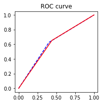
AUC = 0.61213、逐步回归选择变量
<class 'statsmodels.iolib.summary.Summary'>
"""
Generalized Linear Model Regression Results
==============================================================================
Dep. Variable: churn No. Observations: 2424
Model: GLM Df Residuals: 2417
Model Family: Binomial Df Model: 6
Link Function: logit Scale: 1.0
Method: IRLS Log-Likelihood: -1012.7
Date: Fri, 15 Jun 2018 Deviance: 2025.4
Time: 17:51:02 Pearson chi2: 2.26e+03
No. Iterations: 7
================================================================================
coef std err z P>|z| [0.025 0.975]
--------------------------------------------------------------------------------
Intercept 6.4997 2.136 3.043 0.002 2.314 10.686
duration -0.2382 0.011 -21.227 0.000 -0.260 -0.216
peakMinDiff -0.0029 0.000 -7.918 0.000 -0.004 -0.002
AGE -0.0195 0.004 -4.760 0.000 -0.028 -0.011
subscriberID -5.015e-08 2.84e-08 -1.765 0.078 -1.06e-07 5.54e-09
peakMinAv 0.0007 0.000 1.789 0.074 -6.88e-05 0.002
incomeCode 0.0054 0.003 1.660 0.097 -0.001 0.012
================================================================================
"""
ROC曲线: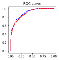
AUC = 0.8974
膨胀系数:
subscriberID     1.006376917076832

AGE      1.0539373172811175

incomeCode       1.0233464772559815

duration         1.0383978966834935

peakMinAv        1.0380990598521813

peakMinDiff      1.036565610813066