以MNIST数据集用tensorflow写个lenet-5卷积神经网络

lenet-5网络的结构可以参考这个链接,这个算法是比较旧的一种算法了，写出来主要是为了提高自己的工程实现能力

https://baijiahao.baidu.com/s?id=1585076668733448115&wfr=spider&for=pc

这个代码改进点：

1、在卷积层和全连接的地方使用的激活函数是relu而不是tanh或者sigmoid

2、在进行padding时候我们进行边界填充

3、使用softmax函数获取各个类别概率

具体就看代码和结果图吧，都有注释

# -*- coding: utf-8 -*-
import matplotlib.pyplot as plt
import numpy as np
import tensorflow as tf
from tensorflow.contrib.learn.python.learn.datasets.mnist import read_data_sets
from matplotlib.font_manager import FontProperties
import matplotlib
font = FontProperties(fname=r"c:\windows\fonts\simsun.ttc", size=14)
zhfont1 = matplotlib.font_manager.FontProperties(fname=r'c:\windows\fonts\simsun.ttc')
#定义回话
sess = tf.Session()
#定义参数
tf.flags.DEFINE_string("data_dir", 'temp', "定义数据路径")
tf.flags.DEFINE_integer("batch_size",100,"定义一次训练有多少个")
tf.flags.DEFINE_float("learing_rates",0.05,"学习率")
tf.flags.DEFINE_integer("evaluation_size",1500,"一次测试集大小")
tf.flags.DEFINE_integer("num_channels",1,"图片通道，黑白的这里我们只有一个")
tf.flags.DEFINE_integer("generations",500,"迭代步数")
tf.flags.DEFINE_integer("eval_ervery",5,"选择每五步打印一次信息")
FLAGS = tf.flags.FLAGS
#load data
#################
def load_data(dir):
    #读取数据
    mnist=read_data_sets(dir)
    #将图片转化为28*28的格式
    train_data=np.array([np.reshape(x,(28,28)) for x in mnist.train.images])
    test_data=np.array([np.reshape(x,(28,28)) for x in mnist.test.images])
    #读入标签数据
    train_labels=mnist.train.labels
    test_labels=mnist.test.labels
    return train_data,test_data,train_labels,test_labels

train_xdata,test_xdata,train_labels,test_labels=load_data(FLAGS.data_dir)
###Parameters
###定义参数
global_step=tf.Variable(0)
#每五步学习率进行一次0.9缩减的缩减
learing_rates = tf.train.exponential_decay(FLAGS.learing_rates, global_step, 5, 0.9, staircase=True)     #生成学习率
#确定图片的宽和高
image_width=train_xdata[0].shape[0]
image_height=train_xdata[0].shape[1]
#确定有几个类被
target_size=max(train_labels)+1
#确定各个卷积层要提取的体征数
conv1_features=25
conv2_features=50
#确定pooling窗口的大小
max_pool_size1=2
max_pool_size2=2
#确定全连接的节点
fully_connected_size1=100
##构造变量[行，宽，高，通道数]
x_input_shape=[FLAGS.batch_size,image_width,image_height,FLAGS.num_channels]
x_input=tf.placeholder(tf.float32,shape=x_input_shape)
y_target=tf.placeholder(tf.int32,shape=(FLAGS.batch_size))
#定义测试集变量
eval_input_shape=(FLAGS.evaluation_size,image_width,image_height,FLAGS.num_channels)
eval_input=tf.placeholder(tf.float32,shape=eval_input_shape)
eval_target=tf.placeholder(tf.int32,shape=(FLAGS.evaluation_size))
#定义卷积核
conv1_weight=tf.Variable(tf.truncated_normal([4,4,FLAGS.num_channels,conv1_features],stddev=0.1,dtype=tf.float32))
conv1_bias=tf.Variable(tf.zeros([conv1_features],dtype=tf.float32))
conv2_weight=tf.Variable(tf.truncated_normal([4,4,conv1_features,conv2_features],stddev=0.1,dtype=tf.float32))
conv2_bias=tf.Variable(tf.zeros([conv2_features],dtype=tf.float32))
#构建全连接层的权重和B
resulting_width=image_width//(max_pool_size1 * max_pool_size2)
resulting_heigh=image_height//(max_pool_size1*max_pool_size2)
#构建权值
full_input_size=resulting_heigh*resulting_width*conv2_features
full1_weight=tf.Variable(tf.truncated_normal([full_input_size,fully_connected_size1],stddev=0.1,dtype=tf.float32))
full1_bias = tf.Variable(tf.truncated_normal([fully_connected_size1],stddev=0.1,dtype=tf.float32))
full2_weight=tf.Variable(tf.truncated_normal([fully_connected_size1,target_size],stddev=0.1,dtype=tf.float32))
full2_bias=tf.Variable(tf.truncated_normal([target_size],stddev=0.1,dtype=tf.float32))
#开始定义模型
def conv_net(input_data):
    #首先定义一下卷积层，池化层，padding
    #定义一下窗口的移动间隔和padding操作
    conv1=tf.nn.conv2d(input_data,conv1_weight,strides=[1,1,1,1],padding="SAME")
    #使用relu作为我们的激活函数
    relu1=tf.nn.relu(tf.nn.bias_add(conv1,conv1_bias))
    #使用max做为池化操作
    max_pool1=tf.nn.max_pool(relu1,ksize=[1,max_pool_size1,max_pool_size1,1],strides=[1,max_pool_size1,max_pool_size1,1],padding="SAME")
    #定义第二层
    #CONV-RELU-MAXPOOL
    conv2=tf.nn.conv2d(max_pool1,conv2_weight,strides=[1,1,1,1],padding="SAME")
    relu2=tf.nn.relu(tf.nn.bias_add(conv2,conv2_bias))
    max_pool2=tf.nn.max_pool(relu2,ksize=[1,max_pool_size2,max_pool_size2,1],strides=[1,max_pool_size2,max_pool_size2,1],padding="SAME")
    #装换成1*N的全连接
    full_conv_shape=max_pool2.get_shape().as_list()
    full_shape = full_conv_shape[1] * full_conv_shape[2] * full_conv_shape[3]
    flat_output = tf.reshape(max_pool2, [full_conv_shape[0], full_shape])
    #第一层全连接输出
    full_connected1 = tf.nn.relu(tf.add(tf.matmul(flat_output, full1_weight), full1_bias))
    #第二层全连接输出
    full_model_output = tf.add(tf.matmul(full_connected1, full2_weight), full2_bias)

    return full_model_output
#定义模型的训练集合测试集的输出
model_output=conv_net(x_input)
test_model_output=conv_net(eval_input)
# 定义损失函数,使用softmax回归
loss = tf.reduce_mean(tf.nn.sparse_softmax_cross_entropy_with_logits(logits=model_output,labels=y_target))

#获取样本对应10个数字中各个的概率
predict=tf.nn.softmax(model_output)
test_predict=tf.nn.softmax(test_model_output)
#这里我们写个准确率损失函数
def get_accuracy(logit,targets):
    #选取在十个类别中最大的数字概率就是
    batch_prediction=np.argmax(logit, axis=1)
    num_correct=np.sum(np.equal(batch_prediction,targets))
    return 100. * num_correct/batch_prediction.shape[0]
#定义训练步骤
#参数优化的方式，随机梯度方式
optimizer=tf.train.GradientDescentOptimizer(learing_rates)
#参数优化方式ADAM方式
#optimizer=tf.train.AdamOptimizer(learing_rates)
train_step=optimizer.minimize(loss)
#变量初始化
init = tf.initialize_all_variables()
sess.run(init)
#定义训练过程
#定义训练过程，并对
train_loss=[]
train_acc=[]
test_acc=[]
for i in range(FLAGS.generations):
    rand_index=np.random.choice(len(train_xdata),FLAGS.batch_size)
    rand_x = train_xdata[rand_index]
    rand_x = np.expand_dims(rand_x, 3)
    rand_y = train_labels[rand_index]
    # 定义输入变量和输入数据映射
    train_dict={x_input:rand_x,y_target:rand_y}
    sess.run(train_step, feed_dict=train_dict)
    train_loss_temp, train_pre_temp = sess.run([loss, predict], feed_dict=train_dict)
    train_acc_temp = get_accuracy(train_pre_temp, rand_y)
    if (i + 1) % FLAGS.eval_ervery == 0:
        eval_index = np.random.choice(len(test_xdata), size=FLAGS.evaluation_size)
        eval_x = test_xdata[eval_index]
        eval_x = np.expand_dims(eval_x, 3)

        eval_y = test_labels[eval_index]
        test_dict = {eval_input: eval_x, eval_target: eval_y}
        test_preds = sess.run(test_predict, feed_dict=test_dict)
        test_acc_temp = get_accuracy(test_preds, eval_y)
        # 将损失和准确率保存
        train_loss.append(train_loss_temp)
        train_acc.append(train_acc_temp)
        test_acc.append(test_acc_temp)

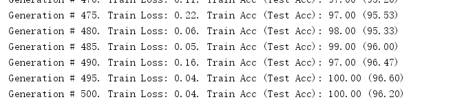
        acc_and_loss = [(i + 1), train_loss_temp, train_acc_temp, test_acc_temp]
        acc_and_loss = [np.round(x, 2) for x in acc_and_loss]
        print('Generation # {}. Train Loss: {:.2f}. Train Acc (Test Acc):{: .2f} ({:.2f})'.format(*acc_and_loss))
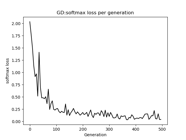
#画图
eval_indices=range(0,FLAGS.generations,FLAGS.eval_ervery)

plt.plot(eval_indices,train_loss,"")
plt.title("GD:softmax loss per generation")
plt.xlabel("Generation")
plt.ylabel("softmax loss")
plt.legend(prop=zhfont1)
plt.show()
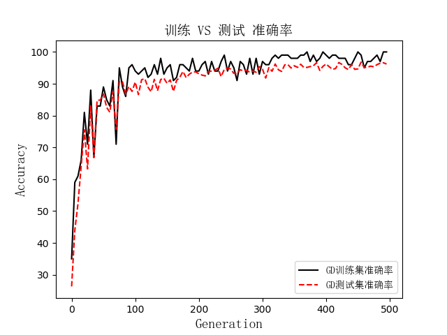
#准确率
# Plot train and test accuracy
plt.plot(eval_indices, train_acc, '', label='GD训练集准确率')
plt.plot(eval_indices, test_acc, 'r--', label='GD测试集准确率')
plt.title('训练 VS 测试 准确率', fontproperties=font)
plt.xlabel('Generation', fontproperties=font)
plt.ylabel('Accuracy', fontproperties=font)
plt.legend(prop=zhfont1)
plt.show()

在迭代到快500次的时候，准确率快达到100%了

训练集合测试集的一个结果比较

损失下降情况，代码中有另外一种参数优化的方式，被我注释了，大家可以测试一下那个迭代的更快